The following implements the implied ERP approach in Professor Damodaran’s post on the The Price of Risk. My intention is to briefly explore its sensitivity to assumptions.
library(tidyverse)
library(scales)

solve_for_R <- function(RF, ER_vector, CP_vector, G2, PV) {

  # Calculate cash flow vector
  CF_vector <- ER_vector * CP_vector

  # Define the objective function
  objective_function <- function(R) {
    # This is effectively two-stage dividend discount model except the initial stage is explicated
    # such that there exists no G1 and G2 refers to the subsequent period of growth

    PV_calculated <- sum(CF_vector[1:5] / (1 + R)^(1:5)) + CF_vector[6] / ((R - G2) * (1 + R)^5)
    return((PV - PV_calculated)^2)
  }

  # Use the optim function to minimize the objective function
  result <- optim(par = RF, fn = objective_function, method = "Brent", lower = -1, upper = 2)

  return(result$par)
}

RF <- 0.04 # I have rounded his riskfree rate of 3.97% to 4.00%
ER_vector <- c(217.8, 245.2, 273.7, 295.1, 308.9, 324.9) # A. Damodaran's earnings vector
CP_vector <- c(0.84, 0.82, 0.80, 0.78, 0.77, 0.77) # Cash payout ratios
G2 <- 0.04 # His model sets the stable growth equal to the RF rate
PV <- 4600 # I rounded 4588.96 to 4,600

implied_equity <- solve_for_R(RF, ER_vector, CP_vector, G2, PV)
implied_ERP <- implied_equity - RF

# Number of simulations
n_simulations <- 10000
coeff_variation <- 0.10 # Arbitrarily suggesting that COV of 10% is tight

# Assumed means and standard deviations for inputs
mean_RF <- RF; sd_RF <- RF * coeff_variation
mean_ER <- ER_vector; sd_ER <- ER_vector * coeff_variation
mean_CP <- CP_vector; sd_CP <- CP_vector * coeff_variation
mean_G2 <- G2; sd_G2 <- G2 * coeff_variation
mean_PV <- PV; sd_PV <- PV * coeff_variation

# MC simulation
set.seed(379)
R_values <- replicate(n_simulations,
  solve_for_R(
    # RF = rnorm(1, mean_RF, sd_RF),
    RF = RF,
    ER_vector = rnorm(6, mean_ER, sd_ER),
    CP_vector = rnorm(6, mean_CP, sd_CP),
    G2 = rnorm(1, mean_G2, sd_G2),
    PV = PV
  )
)

# Histogram to visualize the distribution of R values
R_values <- R_values[R_values > 0]
ERP_values <- R_values - RF
ERP_values_mean <- mean(ERP_values)
ERP_values_df <- as_data_frame(ERP_values)

ERP_values_df %>% ggplot(aes(value)) +
    geom_histogram(color = "darkblue", fill = "lightblue") +
    geom_vline(aes(xintercept = ERP_values_mean), color = "darkgreen", size = 1.5) +
    scale_x_continuous(labels = percent_format(0.01)) +
    labs(title = "Implied equity risk premium, ERP (n = 10,000 sims)",
         subtitle = "Under tight assumption dispersion (CV = σ/μ =10%). Green vertical line is the mean.",
         y = "Count") +
    # xlab("X label") +
    # ylab("Count") +
    theme_classic() +
    theme(axis.title = element_blank(),
          axis.text = element_text(size = 12, face = "bold"))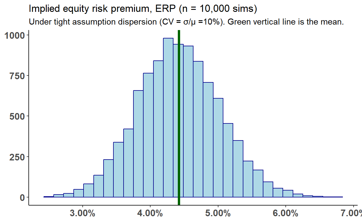
Quick check on the distribution:
[1] 0.08903814kurtosis(ERP_values_df$value)[1] 2.997992quantiles_v <- c(0.01, 0.025, 0.05, 0.1, 0.25, 0.5, 0.75, 0.9, 0.95, 0.975, 0.99)
quantile(ERP_values_df$value, probs = quantiles_v) 1% 2.5% 5% 10% 25% 50%
0.03041180 0.03248300 0.03433620 0.03649075 0.04004356 0.04410500
75% 90% 95% 97.5% 99%
0.04832614 0.05209407 0.05447292 0.05638444 0.05881702 What is the relationship between the sustainable growth rate, G2, and the ERP?
G2_values <- seq(from = 0.02, to = 0.06, by = 0.001)
R_values <- map_dbl(G2_values, function(G2) {
  solve_for_R(
    RF = RF,
    ER_vector = ER_vector,
    CP_vector = CP_vector,
    G2 = G2,
    PV = PV
  )
})

ERP_values <- R_values - RF

G_vs_ERP <-  tibble(
  G2 = G2_values,
  ERP = ERP_values
)

G_vs_ERP %>% ggplot(aes(x = G2, y = ERP)) +
  geom_point() +
  coord_cartesian(ylim = c(.02, .08)) +
  labs(title = "Implied ERP as function of sustainable growth rate, G2",
       subtitle = "Unlike prior/next visualization, predicted vectors are not randomized")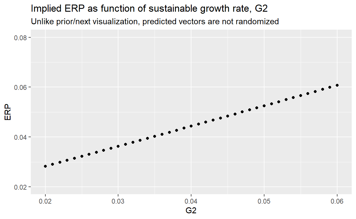
And just for fun, let’s add randomness to the earnings and cash payout vectors:
G2_values <- seq(from = 0.02, to = 0.06, by = 0.001)

R_values <- map(G2_values, function(G2) {
  replicate(30, {
    solve_for_R(
      RF = RF,
      ER_vector = rnorm(6, mean_ER, sd_ER),
      CP_vector = rnorm(6, mean_CP, sd_CP),
      G2 = G2,
      PV = PV
    ) - RF # subtracting RF here inside replicat
  })
})

df <- tibble(
  G2 = G2_values,
  ERP = R_values
) %>% unnest()

model_line <- lm(ERP ~ G2, data = df)
rsq <- summary(model_line)$r.squared
label_R2 <- sprintf("R^2 = %.2f", rsq)

df %>% ggplot(aes(x = G2, y = ERP)) +
  geom_point() +
  coord_cartesian(ylim = c(.02, .08)) +
  geom_smooth(method = "lm", se = TRUE, color = "blue") +
  labs(title = "Restores 10% CV randomness to earnings and payout vectors") +
  annotate("text", x=0.025, y=0.065, label=label_R2, fontface="bold", hjust=0)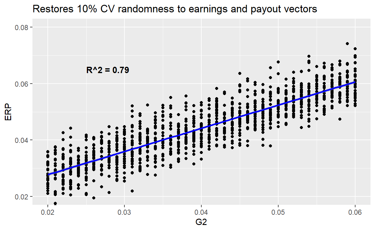
# geom_text(aes(label = label_R2))