I recently completed datacamp’s Intermediate Tidyverse Toolbox skills track. My intention was to get handy with the purrr package, which has a helpful cheat sheet. Purrr requires practice with R’s most versatile data type, the list. In the case of a single list, the essential purrr function is:
map(.x, .f, …); i.e., map(object, function). For example:
d <- map(files, read_csv)
The object can be vector, dataframe or list; recall a dataframe is a list of equal-length vectors.
Here is a traditional loop …
library(tidyverse)
bird_counts <- list(
    c(3,1),
    c(3,8,1,2),
    c(8,3,9,9,5,5),
    c(8,9,7,9,5,4,1,5)
)
class(bird_counts[1]) # returns list
class(bird_counts[[1]]) # returns a numeric vector length 2

# This is a traditional loop ...
bird_sum <- list()
for (i in seq_along(bird_counts)) {
    bird_sum[[i]] <- sum(bird_counts[[i]])
}
… and here is map() replacing the clunky for-loop. Map is a much superior replacement for apply(). Notice how map() returns a list, but map_dbl() returns a numeric vector (of length 1, in this case).
# ... and this is the same result with a single map command:
bird_sum <- map(bird_counts, sum)
str(bird_sum[2]) # = 3 + 8 + 1 + 2
List of 1
$ : num 14str(bird_sum[[2]])
num 14 num 14Since map often operates on a LIST, it is necessary to know how to subset a list and how to set_names() for a list. Better than map(list, function) is the elaborate form:
map(list, ~function(.x))
This gives the same result as map(list, function). The tilde (~) creates a formula that is not evaluated immediately. The .x argument denotes where the (first, and in this case, the only) list element goes inside the function. When we use .x to show where the element goes in the function, we need to put a ~ in front of the function in the second argument of map().
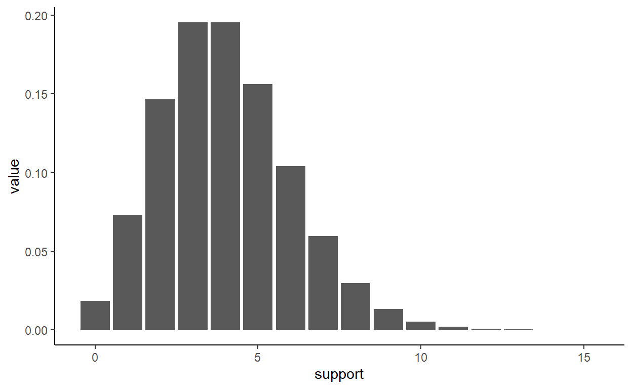
Below is my own pedantic example (not from the course) where I define the poission_pdf() function, then map this function to the integer sequence (aka, support). You can see the whole point of my code is to use map_dbl(support, poisson_pdf)
# function
lam <- 4
poisson_pdf <- function(k){
    lam^k * exp(-lam) / factorial(k)
}

support <- 0:15

poisson_pdf_tbl <- support %>% map_dbl(poisson_pdf) %>% as_tibble(.) %>%
    add_column(support)
poisson_pdf_tbl %>% ggplot(aes(x = support, y = value)) +
    geom_bar(stat = "identity") +
    theme_classic()
Of course above I defined my function, poisson_pdf(), but we can use an anonymous function. Each of the three pipes below gives the same result as above. The first is an anonymous function. The second (and third) is also anonymous but relies on the rlang package for a shortcut with the tilde.
library(scales)
# all three below are effectively identical
1:30 %>% map_dbl(function(k) lam^k * exp(-lam) / factorial(k)) %>% percent(.01) %>% head()
1:30 %>% map_dbl(~lam^. * exp(-lam) / factorial(.)) %>% percent(.01) %>% head()
# When there is only one argument, we can use "." to refer to ".x"
1:30 %>% map_dbl(~lam^.x * exp(-lam) / factorial(.x)) %>% percent(.01) %>% head()
[1] "7.33%"  "14.65%" "19.54%" "19.54%" "15.63%" "10.42%"
[1] "7.33%"  "14.65%" "19.54%" "19.54%" "15.63%" "10.42%"
[1] "7.33%"  "14.65%" "19.54%" "19.54%" "15.63%" "10.42%"
Simulating data and then running a linear model
Map is especially potent because a list’s elements can be lists (e.g., dataframes). Below we use map to create list_of_df which is a list of 3 elements where each element is a 200 × 3 dataframe. Each dataframe contains three columns. The first dataframe has a column, where = “north”; The second dataframe has a column, where = “east.” Then map(~lm(a ~ b, data = .x)) regresses a against b, but it maps the regression formula, lm(), over each of the three dataframes (i.e., they are the list’s elements).
# List of sites north, east, and west
sites <- list("north", "east", "west")

# Create a list of 3 dataframes, each with where, a, and b column
list_of_df <-  map(sites,
  ~data.frame(where = .x,
       a = rnorm(mean = 5, n = 200, sd = 5/2),
       b = rnorm(mean = 200, n = 200, sd = 15)))

lm_results <- list_of_df %>%
    map(~lm(a ~ b, data = .x)) %>% # could also be "data = ."
    map(summary)
So lm_result is a list of 3 (where each of these elements is itself a list of 11 elements that characterizes the regression). For example:
lm_results[[2]]$coefficients
               Estimate Std. Error   t value   Pr(>|t|)
(Intercept) 4.321718041 2.41771085 1.7875248 0.07538217
b           0.003348198 0.01200853 0.2788183 0.78067527
Adverbs and other stuff
The course includes an introduction to troubleshooting with safely() and possibly(). Along with quietly(), these are wrapper functions. Wrapper functions rely on the dot-dot-dot (Some might call this an ellipsis, but apparently it’s a dot-dot-dot). In the chunk below, I define a funciton, var_bhs(), that wraps the base quantile() function:
# Here is artificial L/P data, n = 100. In your opinion, what is the 95.0% HS VaR?
library(tidyverse)
LP_sim <- c(seq(1:94), 96, 99, 103, 108, 114, 121)
quantile(LP_sim, probs = 0.95) # returns 961.5
  95%
96.15
# But if we want to follow Dowd's approach (which is the FRM's), we want:
quantile(LP_sim, probs = 0.95, type = 1)
95%
 96
# Here is my wrapper function; bhs refers to Basic Historical Simulation
var_bhs <- function(...) {
quantile(..., type = 1, names = FALSE)
# %>% format(nsmall = 2)
}
var_bhs(LP_sim, 0.95) # returns 96 which is correct
[1] 96In regard to purrr’s troubleshooting wrappers, walk() returns the input object invisibly, so it is useful in a pipe that wants to perform an action (e.g., print), but then continues to pipe-operate on the same data. The chunk below illustrates the difference between safely() and possibly():
tiny_list <- list(-5, "zero", 0, 3, 12) # contains a negative and a chr

# The won't work at all, object a is not even created. So I won't run it!
# a <- tiny_list %>% map(log)

# Map safely()
# b1 is a list of 5 where each element is a list of 2: result and error
b1 <- tiny_list %>% map(safely(log, otherwise = NA_real_))
b1[[2]]$result; b1[[2]]$error
[1] NA<simpleError in .Primitive("log")(x, base): non-numeric argument to mathematical function># Map safely then transpose()
# b2 is list of 2. The first element is a list of 5 results;
# and the second element is a list of 5 errors
b2 <- tiny_list %>% map(safely(log, otherwise = NA_real_)) %>% transpose()
b2[[1]][[2]]; b2[[2]][[2]]
[1] NA<simpleError in .Primitive("log")(x, base): non-numeric argument to mathematical function>Finally, the code below (most of which is from the course, but the
annotations are mine) did impress me. I am still vexed by how
[ is used, but I found the more intuitive equivalent. About
this subsetting operator, [, see https://stackoverflow.com/questions/57528110/what-does-the-argument-mean-inside-map-df
library(repurrrsive)
names(sw_films) # list of 7 SW films (not sure why not 9), but names() are NULL
NULLsw_films[[1]]$director; sw_films[[7]]$director
[1] "George Lucas"[1] "J. J. Abrams"map_chr(sw_films,"title") # chr vector with 7 elements
[1] "A New Hope"              "Attack of the Clones"
[3] "The Phantom Menace"      "Revenge of the Sith"
[5] "Return of the Jedi"      "The Empire Strikes Back"
[7] "The Force Awakens" [1] "George Lucas" "George Lucas" "George Lucas"
[4] "George Lucas" "Richard Marquand" "Irvin Kershner"
[7] "J. J. Abrams" # ... now a more sophisticated retrieval:
sw_films %>% map_df(`[`, c("title", "director")) # `[` is subsetting the index = c("title", "director")
# A tibble: 7 × 2
  title                   director
  <chr>                   <chr>
1 A New Hope              George Lucas
2 Attack of the Clones    George Lucas
3 The Phantom Menace      George Lucas
4 Revenge of the Sith     George Lucas
5 Return of the Jedi      Richard Marquand
6 The Empire Strikes Back Irvin Kershner
7 The Force Awakens       J. J. Abrams
sw_films %>% map_df(~ .x[.y], c("title", "director")) # is equivalent to this, which is easier for me
# A tibble: 7 × 2
  title                   director
  <chr>                   <chr>
1 A New Hope              George Lucas
2 Attack of the Clones    George Lucas
3 The Phantom Menace      George Lucas
4 Revenge of the Sith     George Lucas
5 Return of the Jedi      Richard Marquand
6 The Empire Strikes Back Irvin Kershner
7 The Force Awakens       J. J. Abrams
# ... and finally a very cool maneuver:
map_chr(sw_films, ~.x[["episode_id"]]) %>% # returns a 7-length chr vector c("4", "2", ... "7")
set_names(map_chr(sw_films, "title")) %>% # then names the chr vector
sort() # and finally sorts the vector
     The Phantom Menace    Attack of the Clones
                    "1"                     "2"
    Revenge of the Sith              A New Hope
                    "3"                     "4"
The Empire Strikes Back      Return of the Jedi
                    "5"                     "6"
      The Force Awakens
                    "7"
Those are my highlights. As I finished the skills track, I’ve already done the subsequent course in the track, Intermediate Functional Programming with purrr. That’s even more purrr, and I’ll collect those notes soon!