How to Process Missing Data

How do we visualize what’s missing? And the art of imputation

I just finished the first course, Dealing with Missing Data in R by Nicholas Tierney, in datacamp’s Intermediate Tidyverse Toolbox skills track. Mr. Tierney is the author of the naniar pacakage. Most of the course applies naniar’s functions.

Okay, missing data is not a glamorous topic. Still, as you know, wrangling is the data scientist’s predominant task. To work with real-world data is to encounter missing data. This course was about:

• Finding and visualizing missing values
• A method for tidy missing data
• How to impute (aka, imputation) missing values

R stores missing values as ‘NA’. Of course, many functions contain a default argument: na.rm = FALSE. Conceptual gotchas include:

• NaN: Not a number; eg, sqrt(-1)
• NULL: “an empty bucket isn’t missing water”
• Inf: infinite; e.g., 10/0

While the ‘NA’ reflects an explicitly missing value (typically as an absent feature), data can be implicitly missing (typically as an absent observation or row). I learned of an interesting typology with respecct to missing data dependence:

• MCAR: Missing Completely at Random. NAs have no association with any observed/unobserved data. Imputation is advisable, and deleting observations is okay (will not bias)
• MAR: Missing at Random: NAs depend on data observed but not data unobserved. Carefully impute, but deleting observations may lead to bias
• MNAR: Missing Not at Random: NAs related to other NAs. Imputation and deletion will bias.

Naniar is the go-to package for missing value workflow

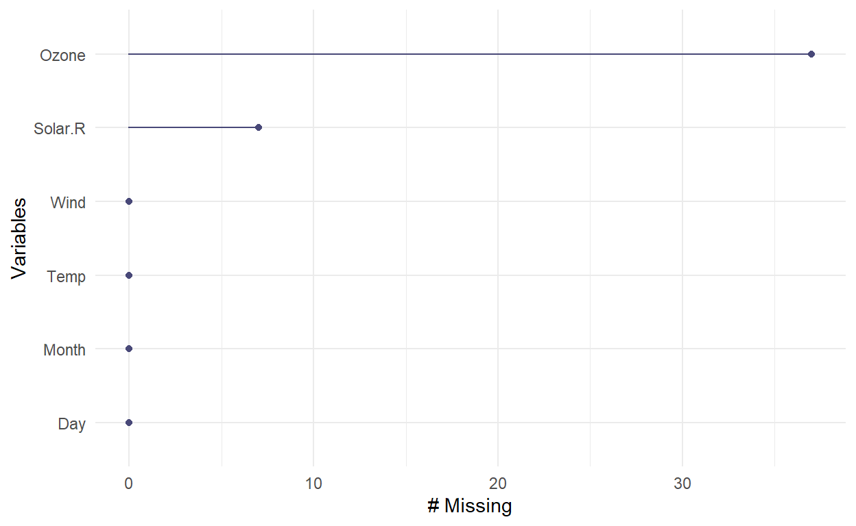
naniar provides at least four numerical summary functions: miss_var_summary(), miss_var_table(), miss_case_summary(), miss_case_table(). But the visualization functions are more fun:

# install.packages("simputation")
library(tidyverse)
library(naniar)
library(simputation)

# vis_miss(airquality) # visdat package
gg_miss_var(airquality) # missing variables

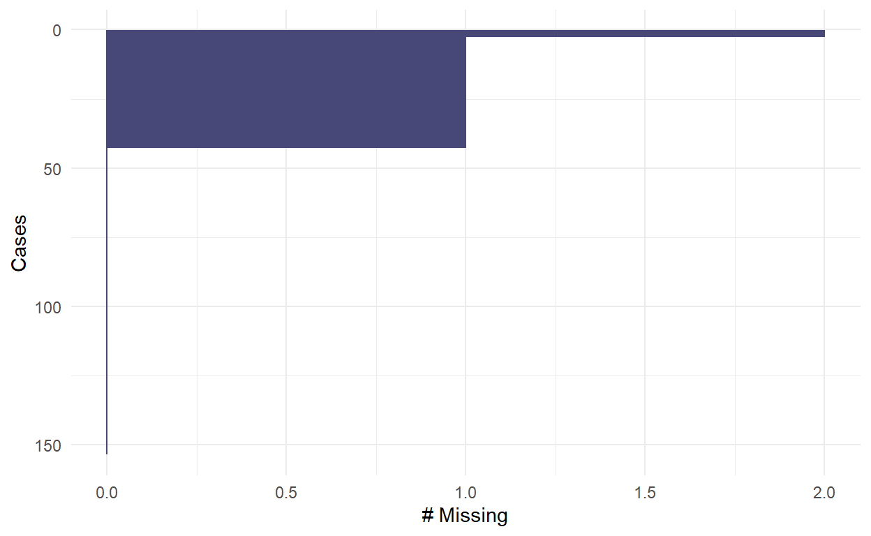
gg_miss_case(airquality) # missing cases

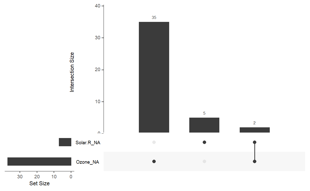
gg_miss_upset(airquality) # an upset plot for missingness patterns

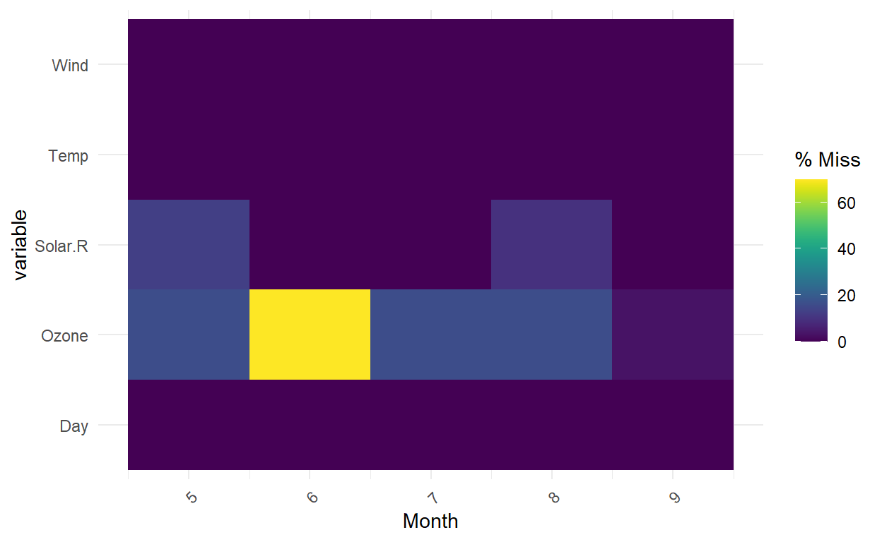
gg_miss_fct(x = airquality, fct = Month) # broken down by facctor

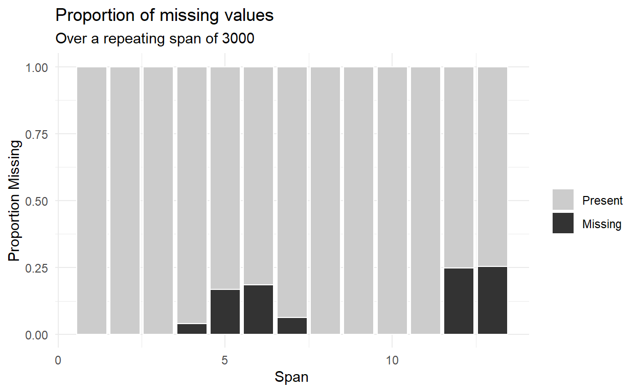
gg_miss_span(pedestrian, hourly_counts, span_every = 3000) #spans of missingness, useful for time series

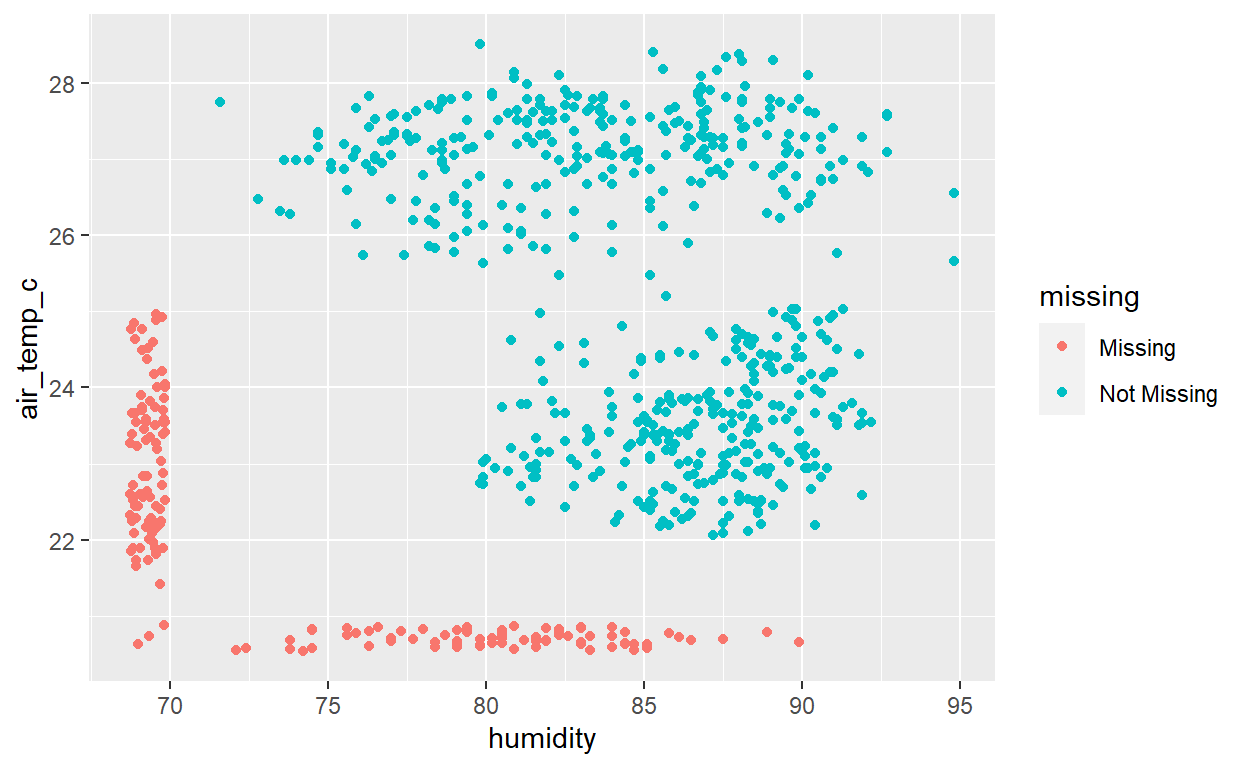
But my favorite visual function is geom_miss_point(). It creatively solves an interesting question, how do you visualize missing values? The standard ggplot() removes missing values and helpfully gives a warning, but you can’t see what’s removed! What geom_miss_point() does is impute a value that is X% below the variable’s minimum value (the default is 10% per the argument prop_below = 0.1). Notice below that there are three cases where both humidity and air_temp_c are missing; i.e., these three points are in the lower-left and we can see them due to argument (default) jitter = 0.05.

oceanbuoys %>% 
    ggplot(aes(x = humidity, y = air_temp_c)) + 
    geom_miss_point()

Shadow matrix and linear regression imputation

To assist in missing data workflow, bind_shadow() creates a “shadow matrix”. Below the original oceanbuoys dataset contains 8 features. the function bind_shadow() doubles the tibble by adding 8 more variables by appending “_NA”: year_NA, latitude_NA, …, wind_ns_NA. The new cells contain only binary indicators: NA or !NA. In this way, “nabular data” is simply the result of the bind_shadow() operation.

Imputation is a vital, deep topic but impute_lm() in the simputation package conveniently performs lm() to impute.

# Impute humidity and air temperature using wind_ew and wind_ns, and track missing values
ocean_imp_lm_wind <- oceanbuoys %>% 
    bind_shadow() %>%
    impute_lm(humidity ~ wind_ew + wind_ns) %>% # from simputation package
    impute_lm(air_temp_c ~ wind_ew + wind_ns) %>%
    add_label_shadow() # adds any_missing colum
    
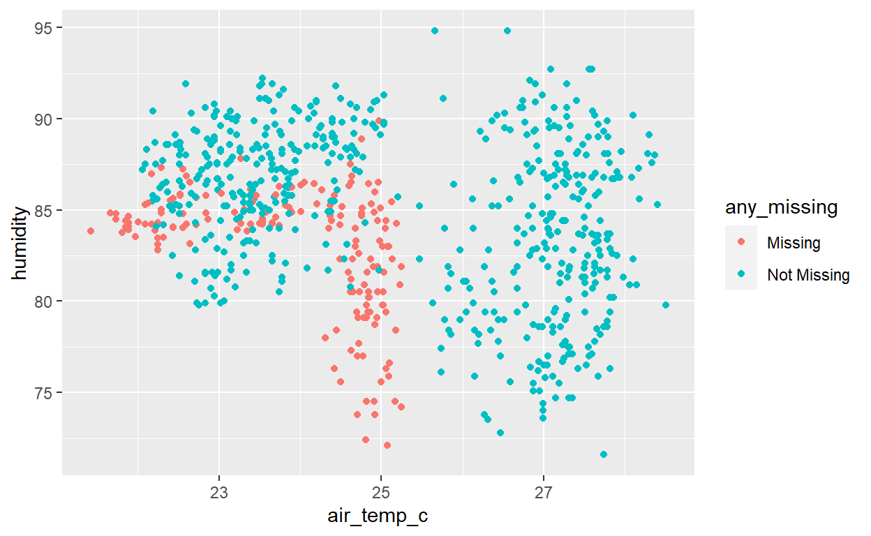
# Plot the imputed values for air_temp_c and humidity, colored by missingness
ggplot(ocean_imp_lm_wind, 
       aes(x = air_temp_c, y = humidity, color = any_missing)) + 
  geom_point()

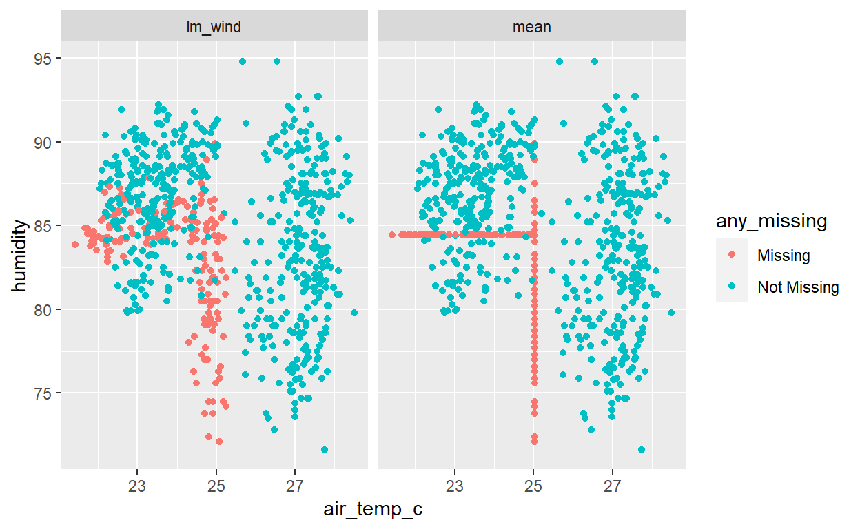
And we can compare the lm() imputations to the naive mean imputations:

ocean_imp_mean <- oceanbuoys %>% # imput means is a bad practice
  bind_shadow() %>% 
  impute_mean_all() %>% 
  add_label_shadow()

# Bind the models together 
bound_models <- bind_rows(mean = ocean_imp_mean,
                          lm_wind = ocean_imp_lm_wind,
                          .id = "imp_model")

# Inspect the values of air_temp and humidity as a scatter plot
ggplot(bound_models, 
       aes(x = air_temp_c, 
           y = humidity, 
           color = any_missing)) +
  geom_point() + 
  facet_wrap(~imp_model)

Thank you Mr. Tierney, I learned a lot! For a deeper exploration, go to the source himself.