Before taking his Advanced Data Visualization with R course, I wanted to refresh my ggplot skills by taking the prior course in the specialization, Data Visualization in R with ggplot2. Both are taught by Collin Paschall of John Hopkins University. This is my final (third) week’s peer-reviewed submission (slightly altered). If you are looking to sharpen your ggplot skills, I highly recommend this course; it can be completed in several hours over three weeks. It does presume familiarity with R (the prior course is “Getting Started with Data Visualization in R”), but this course is not difficult. It incorporates many of the excellent tidyverse references. You’ll never get stuck. It delegates much of the grammar of graphics theory to the textbook.
Notes:
- My submission includes a bar plot (#1), line plot (#2), scatterplot (#3), and distribution (#4)
- There is a facet (#3) and annotation (“Bar height is sample size”)
- Colors are often customized; I tend to prefer the fine control of color = rbg()
Exercise 1
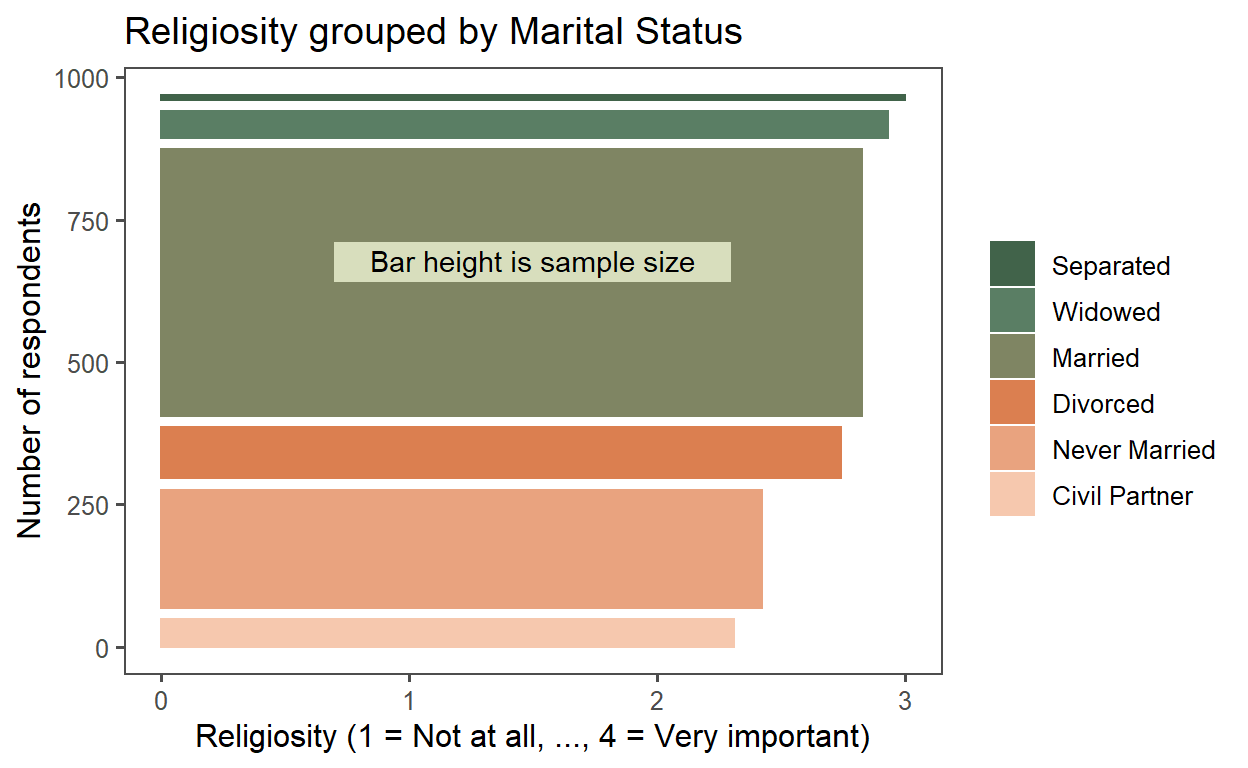
This is a rotated bar chart but the bar widths (which are their vertical height when rotated) represent sample size. The cces data is grouped by Marital Status (i.e., marital). I inverted the pew_region with mutate(pew_religion = 5 - pew_religimp) so that 4 = Very Important. I was curious which groups are the most religious. The highest average is Separated but per the “skinny” bar it’s a small sample. It took some work to get it right; e.g., I had to reorder the factors.
library(tidyverse)
library(ggthemes)
library(forcats)

cces <- read_rds("cces_dh.rds")
cel <- read_rds("cel_dh.rds")

cces <- cces %>% mutate(pew_religion = 5 - pew_religimp)

cces_sum <- cces %>%
    group_by(marstat) %>%
    summarize(
        belief = mean(pew_religion),
        believers = n()) %>%
    arrange(belief)

# Inspired by https://r-graph-gallery.com/81-barplot-with-variable-width.html

cces_sum$marital <- recode(cces_sum$marstat,
       `1` = "Married",
       `2` = "Separated",
       `3` = "Divorced",
       `4` = "Widowed",
       `5` = "Never Married",
       `6` = "Civil Partner")

cces_sum$marital <- fct_reorder(cces_sum$marital, cces_sum$belief, .desc = TRUE)

# Calculate the future positions on the x axis of each bar (left border, central position, right border)
cces_sum$marstat <- as.factor(cces_sum$marstat)
cces_sum$right <- cumsum(cces_sum$believers) + 20*c(0:(nrow(cces_sum)-1))
cces_sum$left <- cces_sum$right - cces_sum$believers

# Plot
cces_sum %>% ggplot(aes(ymin = 0)) +
    geom_rect(aes(xmin = left, xmax = right, ymax = belief, colour = marital, fill = marital)) +
    scale_color_manual(values = c("#41634a", "#5a7e64", "#7f8563", "#db7f50", "#e9a37f", "#f6c8ae")) +
    scale_fill_manual(values = c("#41634a", "#5a7e64", "#7f8563", "#db7f50", "#e9a37f", "#f6c8ae")) +
    ggtitle("Religiosity grouped by Marital Status") +
    xlab("Number of respondents") +
    ylab("Religiosity (1 = Not at all, ..., 4 = Very important)") +
    coord_flip() +
    theme_few() +
    theme(legend.title = element_blank()) +
    annotate(geom = "rect", xmin = 640, ymin = 0.7, xmax = 710, ymax = 2.3, fill = "#d8debd") +
    annotate(geom = "text", x = 680, y = 1.5, label = "Bar height is sample size")
Exercise 2
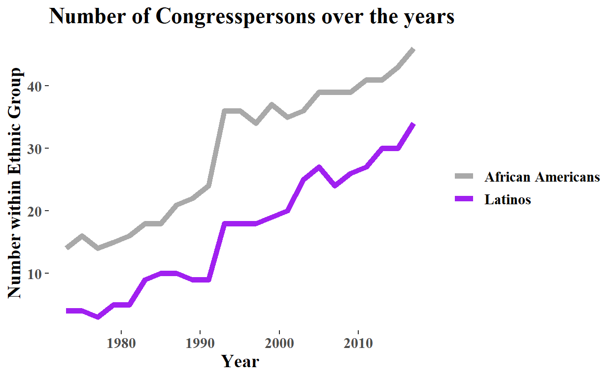
This is a relatively simple geom_line() with ggtheme theme_tufte. I did color Latinos purple to attempt to respectfully match the purple in the Flag of the Hispanic People. As expected, the number of Congresspersons among these two groups grew over the period.
yearly_tbl <- cel %>% group_by(year) %>%
    summarise(
        "African Americans" = sum(afam),
        Latinos = sum(latino),
        total = n()
    )

# yearly_tbl %>% ggplot(aes(x = year)) +
#    geom_line(aes(y = no_afam)) +
#    geom_line(aes(y = no_latino))

yearly_tbl %>%
    pivot_longer(-c(year, total)) %>%
    ggplot(aes(x = year, y = value, color = name)) +
    geom_line(size = 2) +
    scale_color_manual(values = c("dark grey", "purple")) +
    theme_tufte() +
    theme(
        text = element_text(size = 14, face = "bold"),
        legend.title = element_blank()
    ) +
    ggtitle("Number of Congresspersons over the years") +
    xlab("Year") +
    ylab("Number within Ethnic Group")
Exercise 3
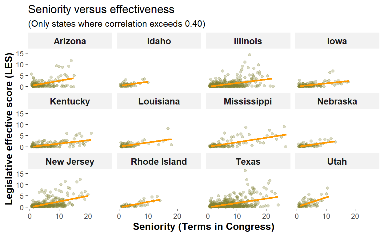
This plot explores whether more tenured congresspersons are more effective. However, I filtered on correlations above 0.40. The colors are custom selected.
cel <- cel %>% group_by(st_name) %>%
    mutate(
        seniority_les = cor(seniority, les)
    )

cel$state_full <- state.name[match(cel$st_name, state.abb)]

cel %>% filter(seniority_les > .42) %>%
    ggplot(aes(x = seniority, y = les)) +
    geom_jitter(color = rgb(.5, .5, .2), alpha = 0.3) +
    geom_smooth(method = "lm", se = FALSE, color = rgb(1, .6, 0), size = 1) +
    labs(
        title = "Seniority versus effectiveness",
        subtitle = "(Only states where correlation exceeds 0.40)",
        x = "Seniority (Terms in Congress)",
        y = "Legislative effective score (LES)") +
    theme(
        plot.title = element_text(size = 14),
        axis.title = element_text(face = "bold", size = 12),
        strip.text.x = element_text(face = "bold", size = 11),
        strip.background = element_rect(fill = rgb(.95, .95, .95)),
        panel.background = element_blank()
    ) +
    facet_wrap(~state_full)
Exercise 4
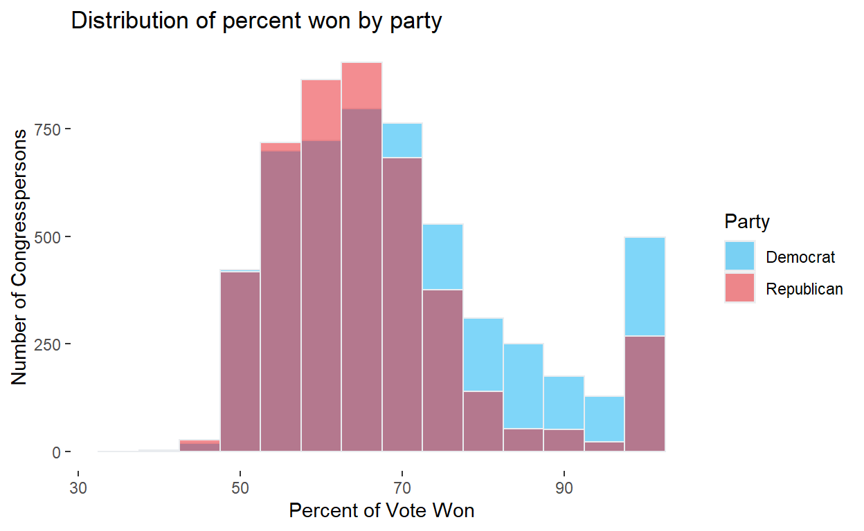
I was curious if the distribution (percent of vote won) appears to be different by party. So these are overlapping histogram. My colors are carefully chosen (via hex) to match each party’s colors and achieve a reddish PURPLE where they overlap.
# cel$female <- as.factor(cel$female)

# cel$female <- as.factor(recode(cel$female, `0` = "Male", `1` = "Female"))
# cel$majority <- as.factor(recode(cel$majority, `0` = "Minority", `1` = "Majority"))

cel$dem <- as.factor(recode(cel$dem, `0` = "Republican", `1` = "Democrat"))

cel %>% rename(Party = dem) %>%
    ggplot(aes(x=votepct, fill = Party)) +
    geom_histogram(binwidth = 5, color="#e9ecef", alpha=0.5, position = 'identity') +
    scale_fill_manual(values=c("#00AEF3", "#E81B23")) +
    labs(
        title = "Distribution of percent won by party",
        x = "Percent of Vote Won",
        y = "Number of Congresspersons") +
    theme(
        panel.background = element_blank(),
    )