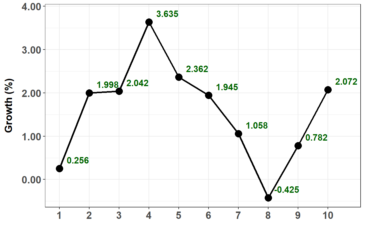
David's (BT) data blog: BT PQ P1.T2.20.25 (SET) Long-horizon AR(p) MA(q) forecasts

20.25.1. Below is plotted the monthly growth rate of a new cryptocurrency over the prior ten months. Two months ago, the growth rate was +0.782%. Last month, the growth rate was +2.072%. We will omit the percentage symbol (%) and assume the growth rates are percentages; specifically, Y(9) = Y(t-2) = +0.782 and Y(10) = Y(t-1) = +2.072

*** plot goes here ***

Your colleagues have determined that the best model for this series is an AR(2) model which is given by Y(t) = ẟ + ϕ(1)*Y(t-1) + ϕ(2)*Y(t-2) + ε(t). In this instance of the model, the intercept is 0.40, the first AR parameter is 0.50 and the second AR parameter is 0.30; specifically, the model is given by Y(t) = 0.40 + 0.50*Y(t-1) + 0.30*Y(t-2) + ε(t). Please note that the intercept of 0.40 here represents 0.40% such that, in decimal terms, the model is given by Y(t) = 0.0040 + 0.50*Y(t-1) + 0.30*Y(t-2) + ε(t) where Y(t-2) = 0.007820 and Y(t-1) = 0.020720 but the AR parameters remain 0.50 and 0.30.

Note that we can markdown/LaTex to render the math. For example, where $ signifies inline LaTex, $$ signifies new line such that the AR(2) is given by \[Y_t =\delta + \phi_1Y_{t-1} +\phi_2Y_{t-2}+\epsilon_t\]

library(tidyverse)
set.seed(13)

AR_param_1 = 0.5
AR_param_2 = 0.3
AR_intercept = 0.4
AR_n <- 10
AR_LR <- AR_intercept/(1- AR_param_1 - AR_param_2)

theme_set(theme_bw())

# arima.sim model c(p, d, q)
# p = AR order
# d = difference
# q = MA order
# Generate an AR(2) with parameters, AR_param_1 and AR_param_2
# Not this: AR <- arima.sim(model=list(order=c(2,0,0), ar = c(AR_param_1, AR_param_2)), n = AR_n) + AR_intercept
AR <- arima.sim(model=list(order=c(2,0,0), ar = c(AR_param_1, AR_param_2)), n = AR_n, mean = AR_intercept)

AR <- round(AR, digits = 3)
AR_tb <- AR %>% as_tibble() %>% rowid_to_column()

# reduced to 80% on copy/paste
AR_tb %>% 
  ggplot(aes(rowid, x)) + 
  ylab("Growth (%)") +
  theme(
    text = element_text(family = "Calibri"), 
    axis.title.x = element_blank(),
    axis.title.y = element_text(size = 13, face = "bold", margin = margin(0,10,0,0)),
    axis.text = element_text(size = 13, face = "bold")
  ) +
  geom_line(size = 1) +
  geom_point(size = 4) + 
  scale_x_continuous(breaks = seq(1, 10, 1), minor_breaks = NULL) +
  scale_y_continuous(labels = scales::number_format(accuracy = 0.01)) +
  geom_text(aes(label = x), size = 4, color = "darkgreen", fontface = "bold", nudge_y = 0.2, nudge_x = .62)

AR[9] # the ts not the tibble

[1] 0.782

AR[10]

[1] 2.072

AR_11 <- AR_intercept + AR_param_1 * AR[10] + AR_param_2 * AR[9]
AR_12 <- AR_intercept + AR_param_1 * AR_11 + AR_param_2 * AR[10]

AR_tb <- cbind(AR_tb, cat = rep("Past",10))
AR_tb <- AR_tb %>% add_row(rowid = 11, x = AR_11, cat = "projected")
AR_tb <- AR_tb %>% add_row(rowid = 12, x = AR_12, cat = "projected")

AR_tb %>% 
  ggplot(aes(rowid, x, group = cat, color = cat)) +
  geom_line() +
  geom_point(size = 4) +
  # xlim(0, 13)
  # scale_x_discrete(limits = c(0,13), breaks = 1)
  scale_x_continuous(breaks = seq(1, 12, 1), minor_breaks = NULL)

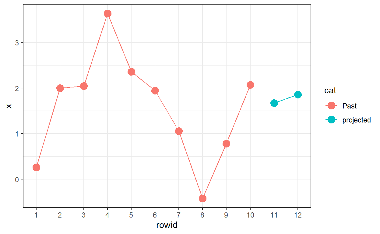
AR_11

[1] 1.6706

AR_12

[1] 1.8569

20.25.3. Long-run mean

20.25.2.Jennifer is an analyst who is deciding which second-order model to fit to her time series dataset. She prefer to fit either an MA(2) or AR(2) model:

MA(2): Y(t) = μ + θ(1)ε(t-1) + θ(2)ε(t-2) + ε(t)
AR(2): Y(t) = ẟ + ϕ(1)Y(t-1) + ϕ(2)Y(t-2) + ε(t)

She is evaluating the models with the same parameters: an intercept of 0.590 and weights of 0.460 and 0.180 such that the two models are specified as follows:

MA(2): Y(t) = 0.590 + 0.460ε(t-1) + 0.180ε(t-2) + ε(t)
AR(2): Y(t) = 0.590 + 0.460Y(t-1) + 0.180Y(t-2) + ε(t)

What are, respectively, the long-run (aka, unconditional) means of these two models?

set.seed(22)

AR2_param_1 = 0.460
AR2_param_2 = 0.180
AR2_intercept = 0.590
AR2_n <- 10

theme_set(theme_bw())

# arima.sim model c(p, d, q)
# p = AR order
# d = difference
# q = MA order
# Generate an AR(2) with parameters, AR_param_1 and AR_param_2
# Not this: AR <- arima.sim(model=list(order=c(2,0,0), ar = c(AR_param_1, AR_param_2)), n = AR_n) + AR_intercept
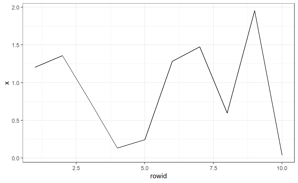
AR2 <- arima.sim(model=list(order=c(2,0,0), ar = c(AR2_param_1, AR2_param_2)), n = AR2_n, mean = AR2_intercept)

AR2 <- round(AR2, digits = 3)
AR2_tb <- AR2 %>% as_tibble() %>% rowid_to_column()

AR2_tb %>% 
  ggplot(aes(rowid, x)) + 
  geom_line()

AR2_11 <- AR2_intercept + AR2_param_1 * AR2[10] + AR2_param_2 * AR2[9]
AR2_12 <- AR2_intercept + AR2_param_1 * AR2_11 + AR2_param_2 * AR2[10]
AR2_13 <- AR2_intercept + AR2_param_1 * AR2_12 + AR2_param_2 * AR2_11
AR2_14 <- AR2_intercept + AR2_param_1 * AR2_13 + AR2_param_2 * AR2_12

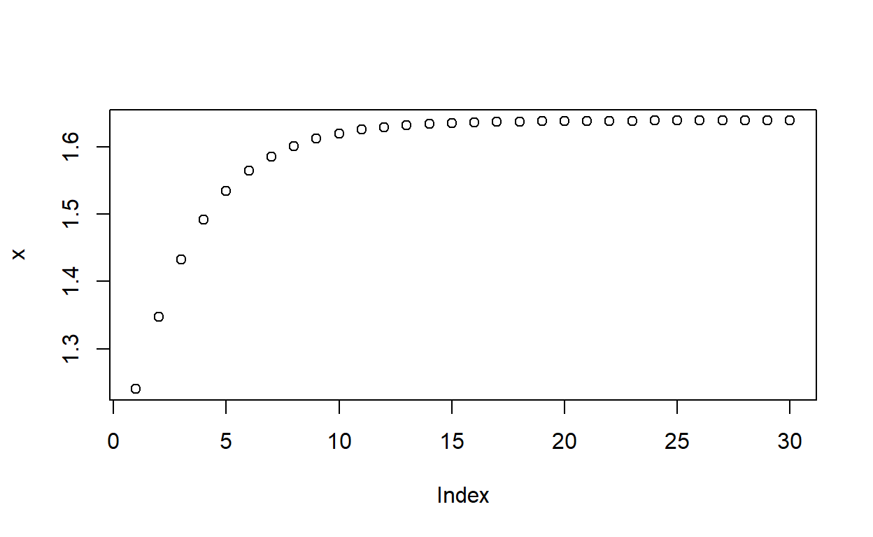
x = vector(mode= "numeric", length = 30)
x[1] = AR2_13
x[2] = AR2_14
for (i in 3:30) {
  x[i] <- AR2_intercept + AR2_param_1 * x[i-1] + AR2_param_2 * x[i-2]
}

plot(x)

AR2_11

[1] 0.95892

AR2_12

[1] 1.037763

AR2_13

[1] 1.239977

AR2_14

[1] 1.347187

x[3]

[1] 1.432902

x[4]

[1] 1.491628

x[5]

[1] 1.534071

x[28]

[1] 1.638846

x[29]

[1] 1.638858

x[30]

[1] 1.638867