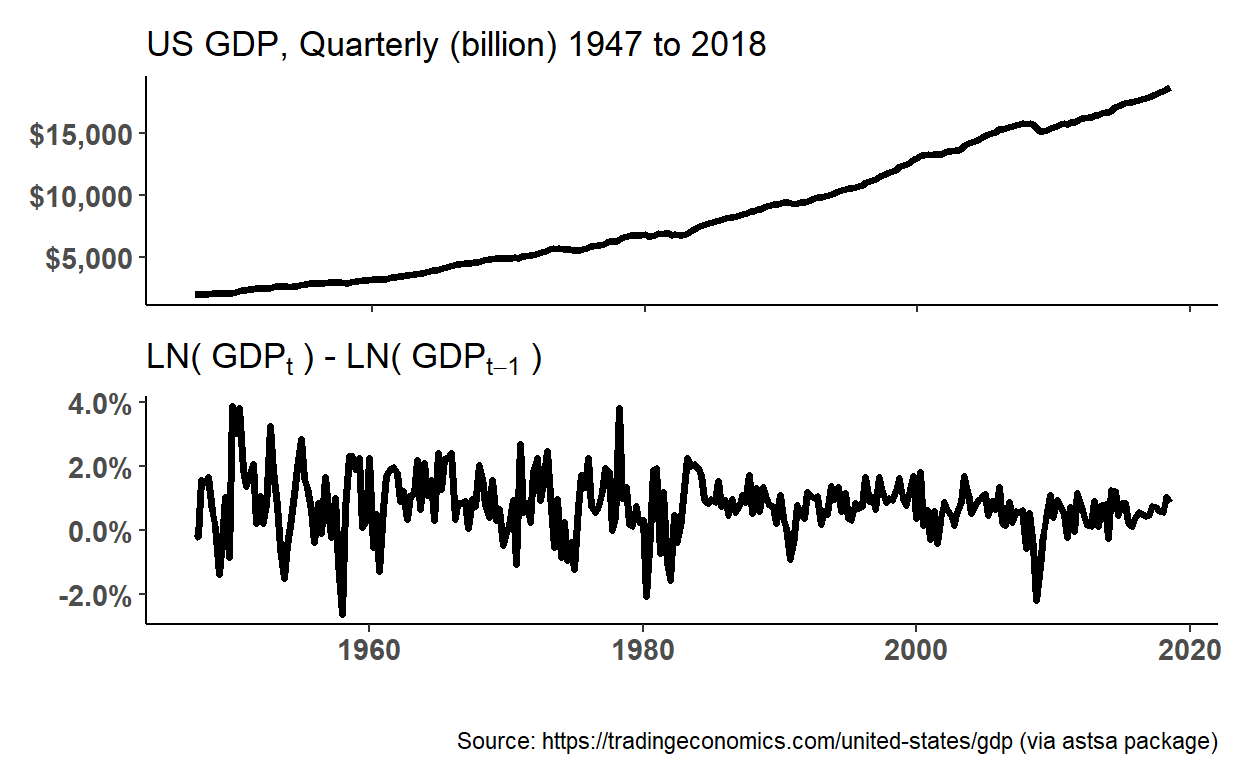
20.24.2. Elizabeth is an economist tasked with modeling quarterly gross domestic product (GDP) in the United States. She starts with the plots displayed below. The raw data is displayed in the upper; she observes this GDP trend is obviously not stationary (why?). She then performs a typical transformation on the raw data: she takes the difference of the natural log of the quarterly GPD values. This plot is displayed in the lower panel. Because LN[GDP(t)] - LN(GDP(t-1)] = LN[GDP(t)/GDP(t-1)], this lower panel plots continuously compounded returns (aka, monthly log returns). First differencing the log returns occasionally renders the non-stationary trend into a stationary process.
library(tidyverse)
library(scales)
library(forecast)
library(tseries)
library(ggthemes)
library(ggfortify)
library(fpp2)
library(gt)
library(astsa)
library(patchwork)
# library(gridExtra)

gdp_log <- diff(log(gdp))

# ts.plot(gdp)
# ts.plot(gdp_log)

p1_gdp <- autoplot(gdp, size = 1.3) + labs(
  title = "US GDP, Quarterly (billion) 1947 to 2018"
) + theme_classic() + theme(
  axis.title.x = element_blank(),
  axis.title.y = element_blank(),
  axis.text.x = element_blank(),
  axis.text.y = element_text(size = 11, face = "bold")
) + scale_y_continuous(labels = dollar_format())

p2_gdp_log <- autoplot(gdp_log, size = 1.3) + labs(
  title = bquote("LN("~GDP[t]~ ") - LN("~GDP[t-1]~")")
) + theme_classic() + theme(
  axis.title.y = element_blank(),
  axis.text.x = element_text(size = 11, face = "bold"),
  axis.text.y = element_text(size = 11, face = "bold")
) + scale_y_continuous(labels = label_percent(accuracy = .1))

patchwork <- p1_gdp / p2_gdp_log
patchwork + plot_annotation(
  caption = "Source: https://tradingeconomics.com/united-states/gdp (via astsa package)"
  )
(on to the Box-Pierce…)
She then fits an autoregressive, AR(1), and moving average, MA(1), model to the log return series. This gives her three models: the log return series (called “diff_logs”), an AR(1) model, and an MA(1) model. She conducts a Box-Pierce test on each of these models; the test of the AR(1) and MA(1) is a test of the residuals. She selects two lags for the test, h = 10 and h = 20. The results of her Box-Pierce test are displayed below.
… Box-Pierce gt table (below) here …
If we assume her desired confidence level is 95.0%, which of the following statements is a TRUE statement with respect to an interpretation of her Box-Pierce test of the three models?
- None of the residuals are white noise; i.e., neither the transformed log returns nor AR(1) nor MA(1) is a candidate model
- The AR(1) is a candidate because its residuals appear to be approximately white noise
- The MA(a) is a candidate because its residuals appear to be approximately white noise
- All of the residuals are white noise; i.e., all three models are candidates
# install.packages("kableExtra")
# install.packages("gapminder")

ar1_gdp_log <- sarima(gdp_log, p = 1, d = 0, q = 0)
initial  value -4.673186
iter   2 value -4.742918
iter   3 value -4.742921
iter   4 value -4.742923
iter   5 value -4.742925
iter   6 value -4.742925
iter   6 value -4.742925
final  value -4.742925
converged
initial  value -4.742229
iter   2 value -4.742234
iter   3 value -4.742245
iter   3 value -4.742245
iter   3 value -4.742245
final  value -4.742245
converged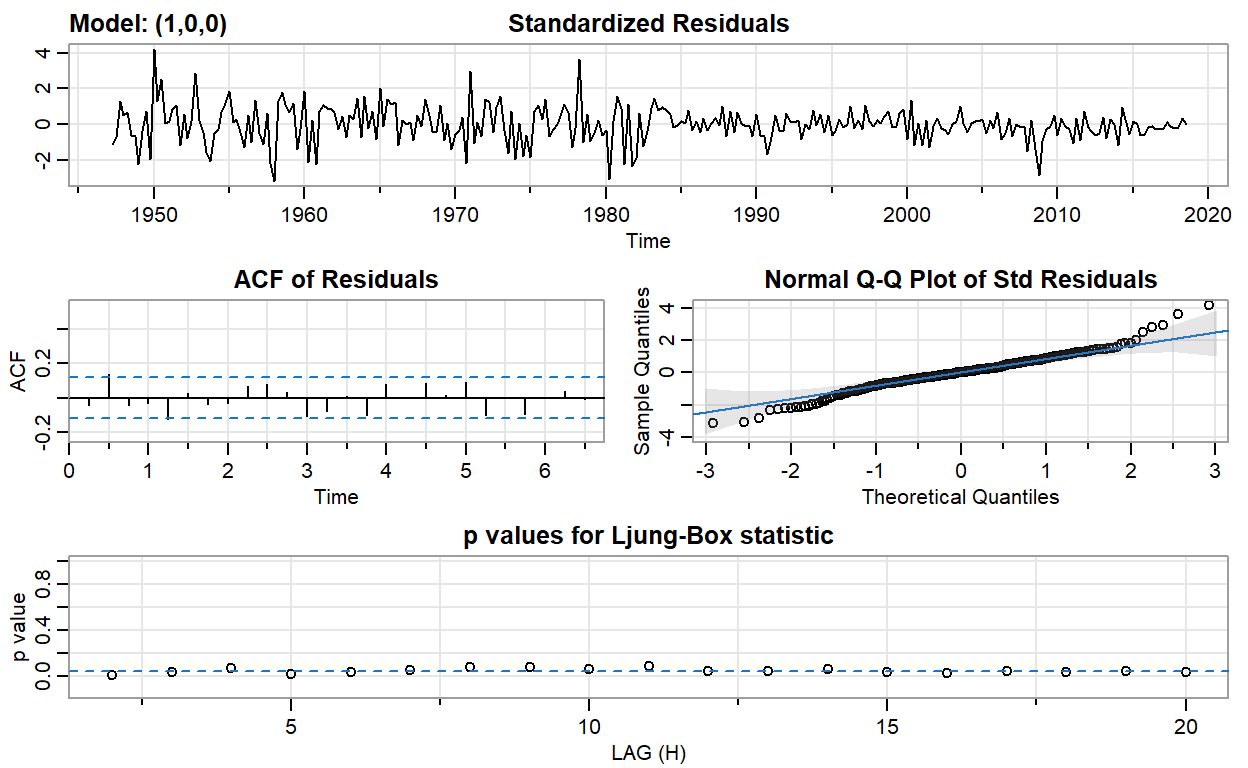
ma1_gdp_log <- sarima(gdp_log, p = 0, d = 0, q = 1)
initial  value -4.672758
iter   2 value -4.716609
iter   3 value -4.723220
iter   4 value -4.723481
iter   5 value -4.723483
iter   5 value -4.723483
iter   5 value -4.723483
final  value -4.723483
converged
initial  value -4.723444
iter   1 value -4.723444
final  value -4.723444
converged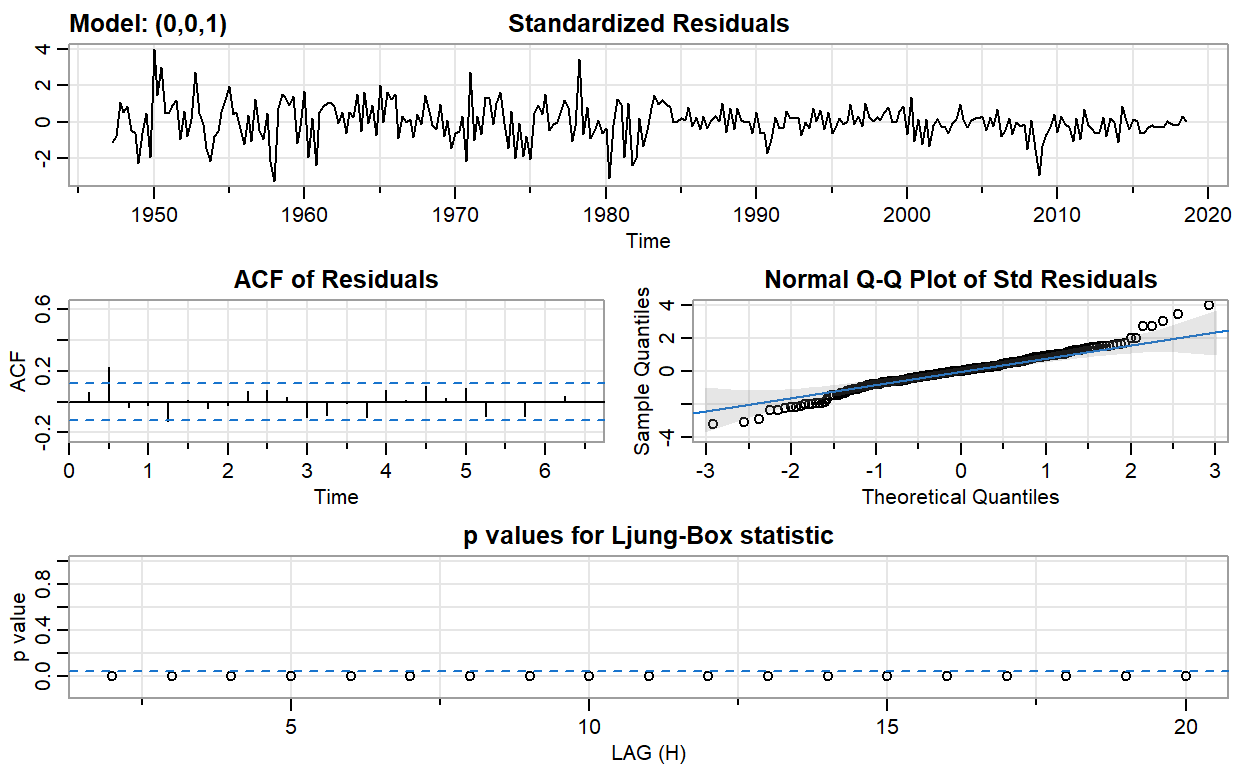
ma2_gdp_log <- sarima(gdp_log, p = 0, d = 0, q = 2)
initial  value -4.672758
iter   2 value -4.749239
iter   3 value -4.750696
iter   4 value -4.750723
iter   5 value -4.750724
iter   6 value -4.750725
iter   7 value -4.750725
iter   7 value -4.750725
iter   7 value -4.750725
final  value -4.750725
converged
initial  value -4.751078
iter   2 value -4.751080
iter   3 value -4.751080
iter   4 value -4.751081
iter   5 value -4.751081
iter   5 value -4.751081
iter   5 value -4.751081
final  value -4.751081
converged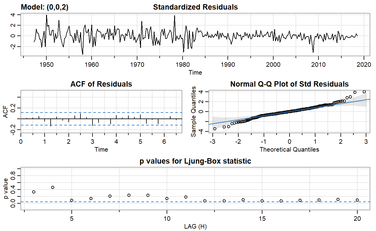
h_values <- c(10, 20)

# diff of logs
model = "diff_logs"
results_log_list <- h_values %>% map(~Box.test(gdp_log, lag = .))
log_statistic <- results_log_list %>% map_dbl("statistic")
log_p.value <- results_log_list %>% map_dbl("p.value")
log_cols <- data.frame(cbind(h_values, log_statistic, log_p.value))
log_all <- cbind(model, log_cols)
log_all <- log_all %>% rename(
  'h (lags)' = h_values,
  statistic = log_statistic,
  'p-value' = log_p.value
)

# AR(1)
model = "AR(1)"
results_ar1_list <- h_values %>% map(~Box.test(ar1_gdp_log$fit$residuals, lag = .))
ar1_statistic <- results_ar1_list %>% map_dbl("statistic")
ar1_p.value <- results_ar1_list %>% map_dbl("p.value")
ar1_cols <- data.frame(cbind(h_values, ar1_statistic, ar1_p.value))
ar1_all <- cbind(model, ar1_cols)
ar1_all <- ar1_all %>% rename(
  'h (lags)' = h_values,
  statistic = ar1_statistic,
  'p-value' = ar1_p.value
)

# MA(1)
model = "MA(1)"
results_ma1_list <- h_values %>% map(~Box.test(ma1_gdp_log$fit$residuals, lag = .))
ma1_statistic <- results_ma1_list %>% map_dbl("statistic")
ma1_p.value <- results_ma1_list %>% map_dbl("p.value")
ma1_cols <- data.frame(cbind(h_values, ma1_statistic, ma1_p.value))
ma1_all <- cbind(model, ma1_cols)
ma1_all <- ma1_all %>% rename(
  'h (lags)' = h_values,
  statistic = ma1_statistic,
  'p-value' = ma1_p.value
)

models_all <- rbind(log_all, ar1_all, ma1_all)
models_gt <- gt(models_all)

models_gt <-
  models_gt %>%
  tab_options(
    table.font.size = 14
  ) %>% tab_style(
    style = cell_text(weight = "bold"),
    locations = cells_body()
  ) %>% tab_style(
    style = cell_text(color = "cadetblue"),
    locations = cells_column_labels(
      columns = vars(model, 'h (lags)', statistic, 'p-value')
    )
  ) %>% tab_header(
    title = md("**Box-Pierce test statistics and p-values**"),
    subtitle = "AR(1) and MA(1) at lags of h = 10 and 20"
  ) %>% fmt_number(
    columns = vars(statistic, 'p-value'),
    decimals = 4
  ) %>% tab_source_note(
    source_note = md("Note: diff_logs = LN[GDP(t)] - LN[GPD(t-1)]")
  ) %>% tab_source_note(
    source_note = md("AR(1) and MA(1) are tests of residuals")
  ) %>% cols_width(
    vars(model, 'h (lags)') ~ px(80),
    vars(statistic, 'p-value') ~ px(90)
  ) %>% cols_label (
    model = md("**model**"),
    'h (lags)' = md("**h (lags)**"),
    statistic = md("**test stat**"),
    'p-value' = md("**p-value**")
  ) %>% cols_align(
    align = "center",
    columns = vars('h (lags)')
  ) %>% tab_options(
    heading.title.font.size = 16,
    heading.subtitle.font.size = 14
  )

models_gt
| Box-Pierce test statistics and p-values | |||
|---|---|---|---|
| AR(1) and MA(1) at lags of h = 10 and 20 | |||
| model | h (lags) | test stat | p-value |
| diff_logs | 10 | 62.6228 | 0.0000 |
| diff_logs | 20 | 80.1439 | 0.0000 |
| AR(1) | 10 | 15.5465 | 0.1134 |
| AR(1) | 20 | 30.3091 | 0.0650 |
| MA(1) | 10 | 24.3689 | 0.0067 |
| MA(1) | 20 | 39.6618 | 0.0055 |
| Note: diff_logs = LN[GDP(t)] - LN[GPD(t-1)] | |||
| AR(1) and MA(1) are tests of residuals | |||