Learning objectives
- Explain mean reversion and calculate a mean-reverting level.
- Define and describe the properties of autoregressive moving average (ARMA) processes.
- Describe the application of AR, MA and ARMA processes.
Let’s load some packages
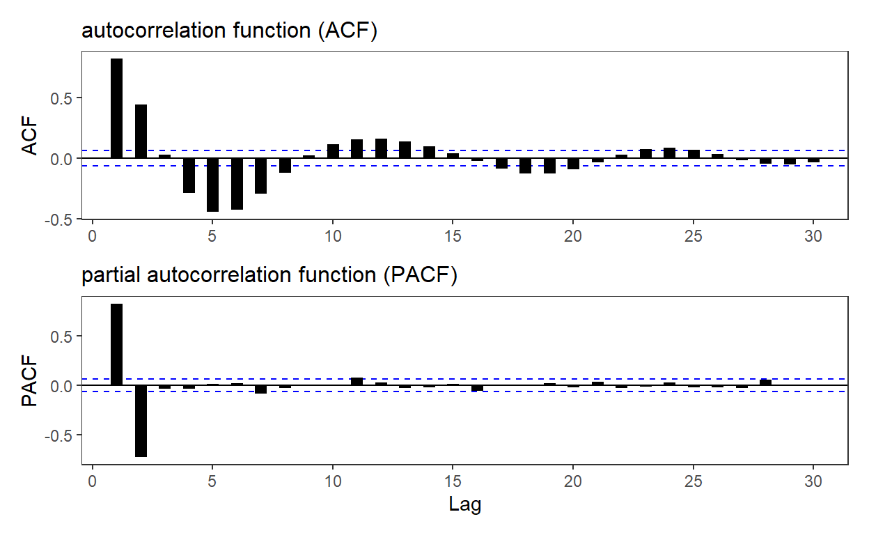
20.23.1. Below are plotted the autocorrelation function (ACF) and partial autocorrelation function (PACF) for a simulated time-series process. Please note that the horizontal dashed blue lines represent the 95.0% confidence interval … Which of the following time-series models is most likely described by these ACF and PACF plots?
set.seed(66)

AR_param_1 = 1.4
AR_param_2 = -0.7
AR_intercept = 0
AR_n <- 1000

theme_set(theme_bw())

# arima.sim model c(p, d, q)
# p = AR order
# d = difference
# q = MA order
# Generate an AR(2) with parameters, AR_param_1 and AR_param_2
AR <- arima.sim(model=list(order=c(2,0,0), ar = c(AR_param_1, AR_param_2)), n = AR_n, mean = AR_intercept)

p3 <- ggAcf(AR) +
  geom_segment(size = 3) +
  labs(
    title = "autocorrelation function (ACF)"
  ) + theme(
    plot.title = element_text(size = 12),
    axis.title.x = element_blank(),
    panel.grid = element_blank()
  )
p4 <- ggPacf(AR) +
  geom_segment(size = 3) +
  labs(
    title = "partial autocorrelation function (PACF)"
  ) + theme(
    plot.title = element_text(size = 12),
    panel.grid = element_blank()
  )

# Please note plot is shrunk to 86% on copy/paste
p3 / p4
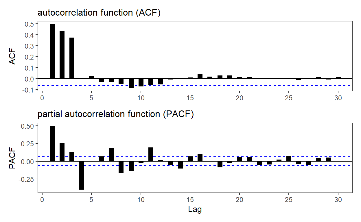
20.23.2. Below are plotted the autocorrelation function (ACF) and partial autocorrelation function (PACF) for a simulated time-series process. Please note that the horizontal dashed blue lines represent the 95.0% confidence interval … Which of the following time-series models is most likely described by these ACF and PACF plots?
set.seed(19)

MA_n = 1000
MA_mean = 0
MA_weight_1 = 0.4
MA_weight_2 = 0.6
MA_weight_3 = 0.8

# # Generate an MA(3) with weights MA_weight_1, MA_weight_2, and MA_weight_3
MA <- arima.sim(model=list(order = c(0,0,3), ma = c(MA_weight_1, MA_weight_2, MA_weight_3)), n = MA_n, mean = MA_mean)

p5 <- ggAcf(MA) +
  geom_segment(size = 3) +
  # geom_hline(yintercept = c(ci2, -ci2), color = "darkblue", linetype = "dashed", size = 2 ) +
  labs(
    title = "autocorrelation function (ACF)"
  ) + theme(
    plot.title = element_text(size = 12),
    axis.title.x = element_blank(),
    panel.grid = element_blank()
  )
p6 <- ggPacf(MA) +
  geom_segment(size = 3) +
  labs(
    title = "partial autocorrelation function (PACF)"
  ) + theme(
    plot.title = element_text(size = 12),
    panel.grid = element_blank()
  )

# Please note plot is shrunk to 86% on copy/paste
p5 / p6
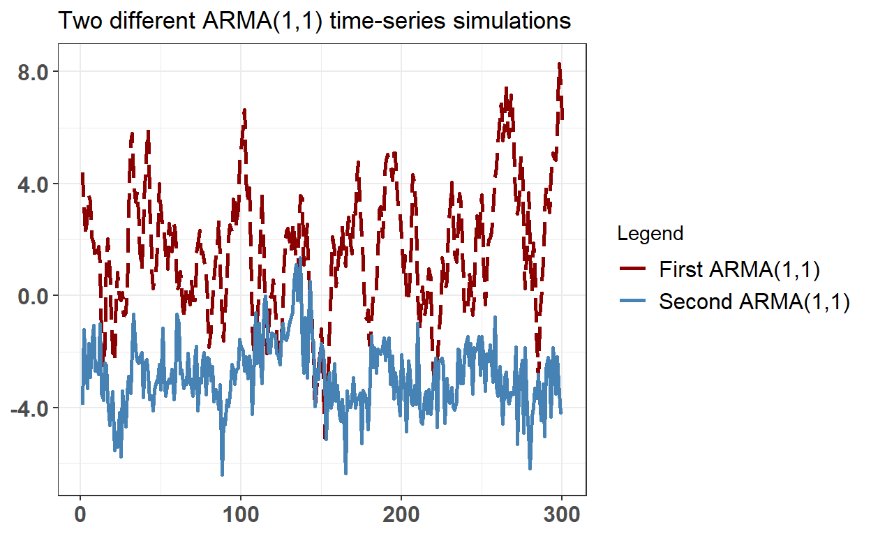
20.23.3. An ARMA(1,1) process evolves according to Y(t) = ẟ + ϕ*Y(t-1) + θ*ε(t-1) + ε(t). The plot below contains two 300-step ARMA(1,1) processes that differ only in their coefficients …
Which of the following statements is TRUE about the two ARMA(1,1) simulations above?
- Both of the ARMA(1,1) processes are likely to exhibit slow decay in both the ACF and PACF
- Both of the ARMA(1,1) processes are likely to cut off sharply at lag 1 in both the ACF and PACF
- The first ARMA(1,1) process (i.e., plotted with a red dashed line) cannot be covariance-stationary
- The unconditional mean of both ARMA(1,1) processes must be zero because all ARMA(1,1) have a long-run mean of zero
library(astsa)
set.seed(9)

ar_11_1 = 0.8
ma_11_1 = 0.6
arma_11_1_mu = 2
sim_n = 300

ar_11_2 = 0.9
ma_11_2 = -0.5
arma_11_2_mu = -3

# ar_22 = c(1.4, -0.6)
# ma_22 = c(0.9, 0.6)

ARMA_11_1 <- arima.sim(model=list(order = c(1, 0, 1), ar = ar_11_1, ma = ma_11_1), n = sim_n) + arma_11_1_mu
ARMA_11_2 <- arima.sim(model=list(order = c(1, 0, 1), ar = ar_11_2, ma = ma_11_2), n = sim_n) + arma_11_2_mu
# ARMA_22 <- arima.sim(model=list(order = c(2, 0, 2), ar = ar_22, ma = ma_22), n = 200)

# ts.plot(ARMA_11, ARMA_22)

time_arma <- bind_cols(ARMA_11_1, ARMA_11_2) %>% rowid_to_column() %>%
  rename(y_ARMA_11_1 = ...1, y_ARMA_11_2 = ...2)


theme_set(theme_bw())

colors <- c("First ARMA(1,1)" = "darkred", "Second ARMA(1,1)" = "steelblue")

time_arma %>% ggplot(aes(x = rowid)) +
  geom_line(aes(y = y_ARMA_11_1, color = "First ARMA(1,1)"), size = 1, linetype = "longdash") +
  geom_line(aes(y = y_ARMA_11_2, color = "Second ARMA(1,1)"), size = 1) +
  scale_y_continuous(labels = scales::number_format(accuracy = 0.1)) +
  theme(
    axis.title.y = element_blank(),
    axis.title.x = element_blank(),
    axis.text.x = element_text(size = 12, face = "bold"),
    axis.text.y = element_text(size = 12, face = "bold"),
    legend.position = "right",
    legend.text = element_text(size = 12)
  ) + labs(
    title = "Two different ARMA(1,1) time-series simulations",
    color = "Legend"
  ) +
  scale_color_manual(values = colors)
arma_11_1_mulr = arma_11_1_mu/(1 - ar_11_1)
arma_11_2_mulr = arma_11_2_mu/(1 - ar_11_2)
# mu_arma_22 = 10
#ARMA_22 <- arima.sim(model=list(order = c(2, 0, 2), ar = c(0.4, 0.2), ma = c(0.5,0.6)), n = 200, mean = mu_arma_22)
# ts.plot(ARMA_22)
# acf2(ARMA_22)
# mean_arma_22 = mu_arma_22/(1 - 0.4 - 0.2)
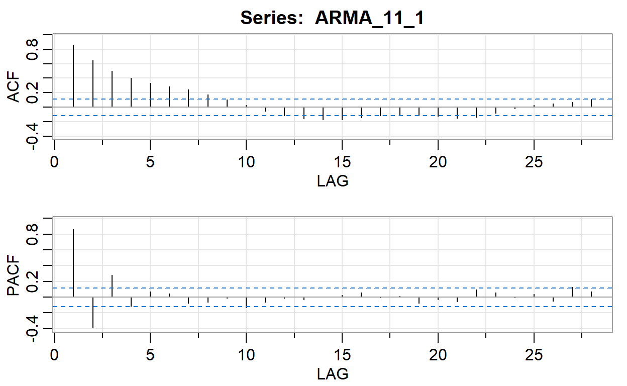
acf2(ARMA_11_1)
     [,1]  [,2] [,3]  [,4] [,5] [,6]  [,7]  [,8]  [,9] [,10] [,11]
ACF  0.86  0.65 0.50  0.40 0.33 0.29  0.24  0.18  0.11  0.03 -0.05
PACF 0.86 -0.39 0.28 -0.11 0.07 0.05 -0.07 -0.06 -0.01 -0.13 -0.06
     [,12] [,13] [,14] [,15] [,16] [,17] [,18] [,19] [,20] [,21]
ACF  -0.12 -0.16 -0.17 -0.17 -0.15 -0.12 -0.10 -0.11 -0.13 -0.15
PACF -0.01 -0.03  0.01  0.03  0.06  0.00  0.01 -0.08 -0.03 -0.05
     [,22] [,23] [,24] [,25] [,26] [,27] [,28]
ACF  -0.14 -0.08 -0.02  0.03  0.05  0.07  0.11
PACF 0.10 0.06 0.00 0.04 -0.05 0.13 0.07acf2(ARMA_11_2)
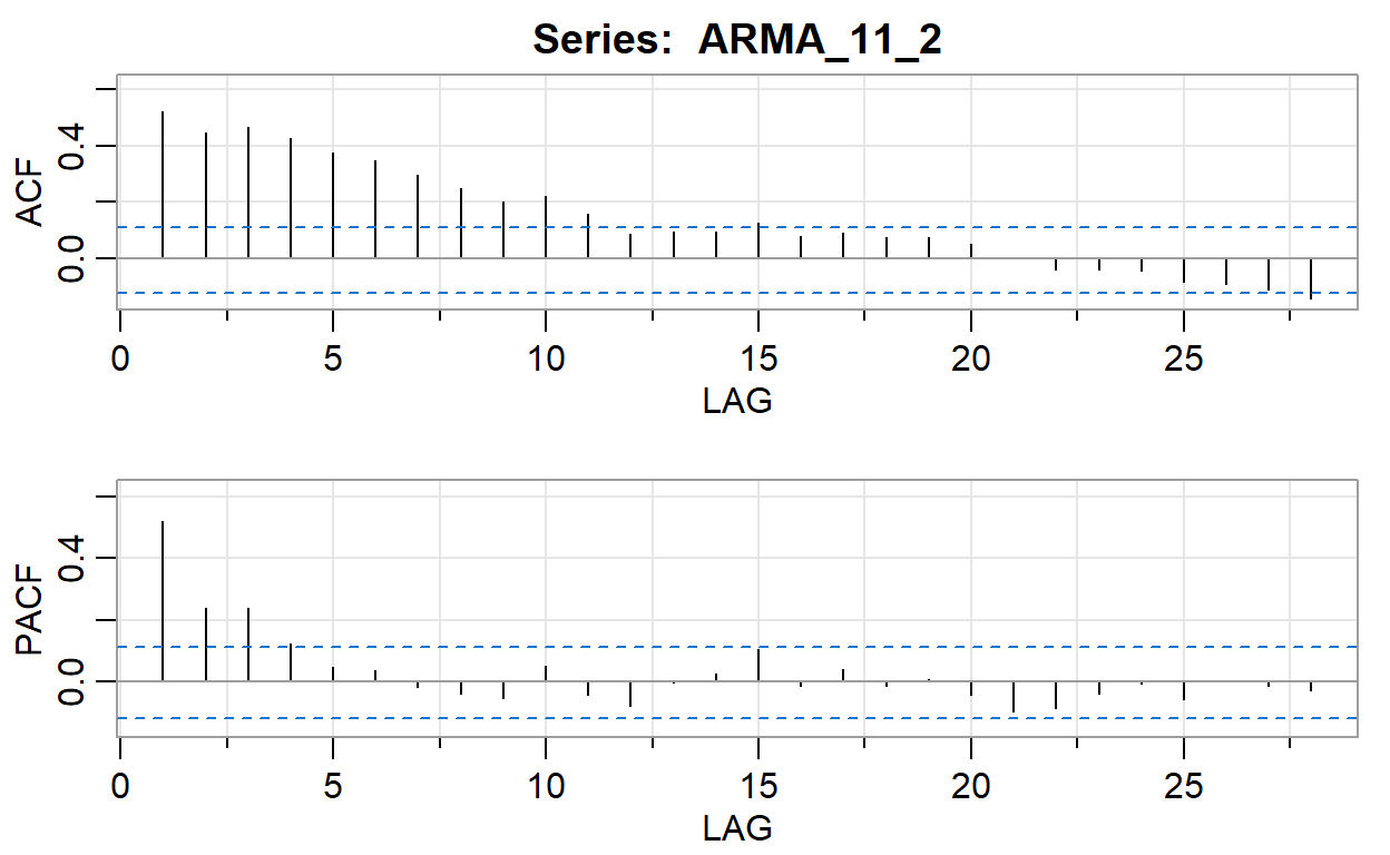
     [,1] [,2] [,3] [,4] [,5] [,6]  [,7]  [,8]  [,9] [,10] [,11]
ACF  0.52 0.45 0.46 0.43 0.37 0.35  0.30  0.25  0.20  0.22  0.16
PACF 0.52 0.24 0.24 0.12 0.05 0.04 -0.02 -0.04 -0.05  0.05 -0.04
     [,12] [,13] [,14] [,15] [,16] [,17] [,18] [,19] [,20] [,21]
ACF   0.09  0.09  0.10  0.13  0.08  0.09  0.08  0.07  0.05  0.00
PACF -0.08  0.00  0.03  0.10 -0.01  0.04 -0.01  0.01 -0.04 -0.09
     [,22] [,23] [,24] [,25] [,26] [,27] [,28]
ACF  -0.04 -0.04 -0.04 -0.08 -0.09 -0.11 -0.14
PACF -0.09 -0.04 -0.01 -0.06  0.00 -0.01 -0.03
end of post