BT PQ P1.T2.20.21.3 White Noise (WN) Process

White noise (WN) is the basic time series building block

A WN process has three three properties:

1. zero mean, but note non-zero means are easily transformed
2. constant and finte variance
3. [The critical property] No autocorrelation or autocovariance

BT PQ P1-T2-20-21-3: White Noise (WN) Process)

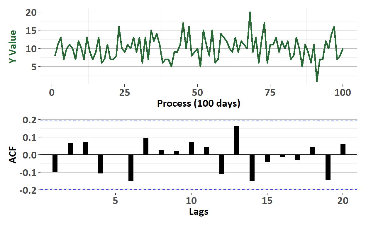
BT 20.21.3. Barbara was delighted to learn that she can easily simulate white noise in R with a single command. She learned that she can use arima.sim(model = list(order = c(0,0,0)), n = 100) to generate white noise with an ARIMA(0,0,0) model over a length of 100 days. She wants the shocks to have a Poisson distribution so she uses the command arima.sim(model = list(order = c(0,0,0)), n = 100, rand.gen = function(n, …) rpois(n, lambda = 10)) which assumes a Poisson distribution. Below is a plot of the white noise (top panel) and its associated autocorrelation function (ACF, bottom panel).

# Simulate a WN model with list(order = c(0, 0, 0))
# white_noise <- arima.sim(model = list(order = c(0,0,0)), n = 100)
# white_noise_1_tb  <- as_tibble(white_noise) %>% rowid_to_column()
# p1 <- ggplot(white_noise_1_tb, aes(x = rowid, y = x)) + geom_line()
# p2 <- ggAcf(white_noise)
# grid.arrange(p1, p2)

library(tidyverse)
library(forecast)
library(patchwork)
library(extrafont)
library(ggthemes)
# library(ggfortify)
# library(cowplot)

set.seed(58)

# Simulate a WN model with list(order = c(0, 0, 0))
# dat_wn <- arima.sim(model = list(order = c(0,0,0)), n = 100)
dat_wn <- arima.sim(model = list(order = c(0,0,0)), n = 100, 
                         rand.gen = function(n, ...) rpois(n, lambda = 10))
dat_wn_tbl <- bind_cols(dat_wn) %>% rowid_to_column() %>% rename(value_y = ...1 )

process_color = "#266935"
p1 <- dat_wn_tbl %>% ggplot(aes(x = rowid, y = value_y)) +
  geom_line(size= 1, color = process_color) +
  ylab("Y Value") +
  xlab("Process (100 days)") + 
  theme_bw() + 
  theme(
    text = element_text(family = "Calibri"),
    plot.title = element_blank(),
    axis.title.x = element_text(size = 14, face = "bold"),
    axis.title.y = element_text(size = 14, face = "bold", color = process_color),
    axis.text.x = element_text(size = 14, face = "bold"),
    axis.text.y = element_text(size = 14, face= "bold"),
    panel.background = element_blank(),
    panel.grid.major.x = element_blank(),
    panel.grid.major.y = element_line(color="grey"),
    panel.border = element_blank()
  )

#p2 <- ggAcf(dat_wn)

p2 <- ggAcf(dat_wn) + 
  xlab("Lags") + 
  theme_bw() +
  geom_segment(size = 3) +
  theme(
    text = element_text(family = "Calibri"),
    plot.title = element_blank(),
    axis.title.x = element_text(size = 14, face = "bold"),
    axis.title.y = element_text(size = 14, face = "bold"),
    axis.text.x = element_text(size = 14, face = "bold"),
    axis.text.y = element_text(size = 14, face= "bold"),
    panel.background = element_blank(),
    panel.grid.major.x = element_blank(),
    panel.grid.major.y = element_line(color="grey"),
    panel.border = element_blank()
  )


# grid.arrange(p1, p2)

p1/p2

s5 <- arima.sim(model = list(order = c(0,0,0)), n = 100, 
                         rand.gen = function(n, ...) rpois(n, lambda = 10))

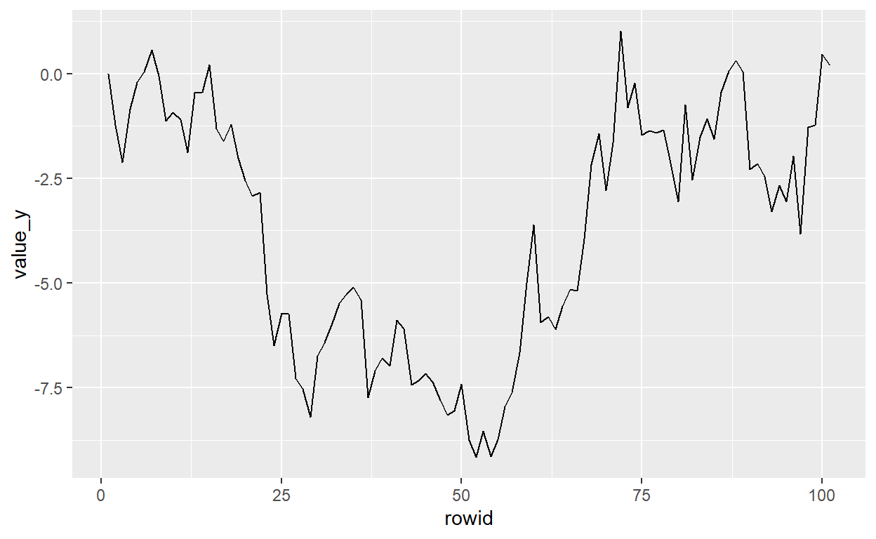
dat_rw <- arima.sim(model = list(order = c(0,1,0)), n = 100)
dat_rw_tbl <- bind_cols(dat_rw) %>% rowid_to_column() %>% rename(value_y = ...1 )
dat_rw_tbl %>% ggplot(aes(x = rowid, y = value_y)) + geom_line()

Is Barbara’s time series model a genuine white noise (WN) process?

1. Yes, Barbara’s simulation is white noise: although the series has a non-zero mean it can easily be defined in terms of a mean-zero error
2. Yes, Barbara’s simulation is white noise: this series has heteroskedasticity and positive auto-covariance which are both valid features of white noise
3. No, Barbara’s simulation is not white noise because white noise must be independent and the lower panel proves this series is not white noise
4. No, Barbara’s simulation is not white noise because white noise requires that she assume the distribution function is normal but the shocks in her series are non-normal