David's (BT) data blog: BT PQ P1-T2-20-17. Univariate regressions cont (2nd set v2)

Learning objectives

Construct, apply, and interpret hypothesis tests and confidence intervals for a single regression coefficient in a regression.
Explain the steps needed to perform a hypothesis test in a linear regression.
Describe the relationship between a t-statistic, its p-value, and a confidence interval.

Let’s load some packages!

library(tidyverse)
library(tidyquant)
library(lubridate)
library(readxl)
library(timetk)
library(tibbletime)
library(quantmod)
library(PerformanceAnalytics)
library(scales)
library(broom)
library(gt)

First question

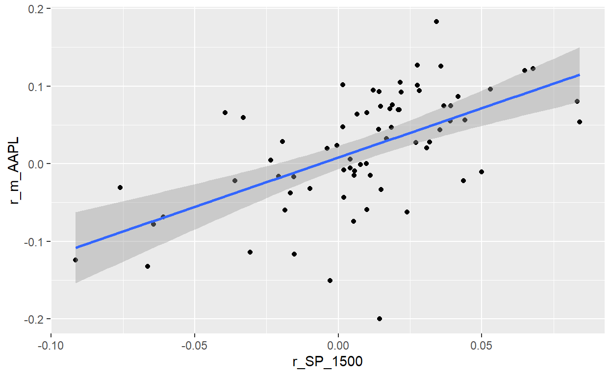
BT 20.17.1. Below the results of a linear regression analysis are displayed. The dataset is monthly returns over a six-year period; i.e., n = 72 months. The gross returns of Apple’s stock (ticker: AAPL) were regressed against the S&P 1500 Index (the S&P 1500 is our proxy for the market). The explanatory variable is SP_1500 and the response (aka, dependent) variable is AAPL.

Question: Which is nearest to the 90.0% confidence interval for the beta of Apple’s (AAPL) stock?

AAPL <- tq_get('AAPL',
               from = "2009-01-01",
               to = "2020-01-01")

SP1500 <- tq_get('SPTM',
               from = "2009-01-01",
               to = "2020-01-01")

AAPL <- AAPL %>% select(date, adjusted)
SP1500 <- SP1500 %>% select(date, adjusted)

AAPL_monthly <- AAPL %>% 
  tq_transmute(select = adjusted, mutate = to.monthly, indexAt = "lastof")
SP1500_monthly <- SP1500 %>% 
  tq_transmute(select = adjusted, mutate = to.monthly, indexAt = "lastof")

AAPL_monthly <- AAPL_monthly %>% mutate(
  r_m_AAPL = log(adjusted/lag(adjusted)))
SP1500_monthly <-SP1500_monthly %>% mutate(
  r_m_SP = log(adjusted/lag(adjusted)))

AAPL_monthly <- AAPL_monthly %>% 
  rename(date_AAPL = date,
         adj_AAPL = adjusted)
SP1500_monthly <- SP1500_monthly %>% 
  rename(date_SP = date,
         adj_SP = adjusted)

both_monthly <- cbind(SP1500_monthly, AAPL_monthly)

both_72 <- both_monthly[-c(1:60), ]
both_72 <- both_72 %>% rename(r_SP_1500 = r_m_SP)
saveRDS(both_72, "t2-20-17-aapl-sp1500.rds")

con <- url("http://frm-bionicturtle.s3.amazonaws.com/david/t2-20-17-aapl-sp1500.rds")
both_72 <- readRDS(con)
close(con)


model_72 <- lm(r_m_AAPL ~ r_SP_1500, data = both_72)
summary(model_72)


Call:
lm(formula = r_m_AAPL ~ r_SP_1500, data = both_72)

Residuals:
      Min        1Q    Median        3Q       Max 
-0.226290 -0.027060  0.002344  0.040667  0.131313 

Coefficients:
            Estimate Std. Error t value Pr(>|t|)    
(Intercept) 0.007969   0.007477   1.066     0.29    
r_SP_1500   1.269627   0.215600   5.889 1.23e-07 ***
---
Signif. codes:  0 '***' 0.001 '**' 0.01 '*' 0.05 '.' 0.1 ' ' 1

Residual standard error: 0.06123 on 70 degrees of freedom
Multiple R-squared:  0.3313,    Adjusted R-squared:  0.3217 
F-statistic: 34.68 on 1 and 70 DF,  p-value: 1.23e-07

p1_model_72 <- both_72 %>% ggplot(aes(r_SP_1500, r_m_AAPL)) +
  geom_point() +
  geom_smooth(method = "lm")

model_72_tidy <- tidy(model_72)

gt_table_model_72 <- gt(model_72_tidy)

gt_table_model_72 <- 
  gt_table_model_72 %>% 
  tab_options(
    table.font.size = 14
  ) %>% 
  tab_style(
    style = cell_text(weight = "bold"),
    locations = cells_body()
  ) %>% 
  tab_header(
    title = "AAPL versus S&P_1500: Gross (incl. Rf) monthly log return",
    subtitle = md("Six years (2014 - 2019), n = 72 months")
  ) %>% 
  tab_source_note(
    source_note = "Source: tidyquant https://cran.r-project.org/web/packages/tidyquant/"
  ) %>% cols_label(
    term = "Coefficient",
    estimate = "Estimate",
    std.error = "Std Error",
    statistic = "t-stat",
    p.value = "p value"
  ) %>% fmt_number(
    columns = vars(estimate, std.error, statistic),
    decimals = 3
  ) %>% fmt_scientific(
    columns = vars(p.value),
  ) %>% 
  tab_options(
    heading.title.font.size = 14,
    heading.subtitle.font.size = 12
  )

gt_table_model_72

AAPL versus S&P_1500: Gross (incl. Rf) monthly log return
Six years (2014 - 2019), n = 72 months
Coefficient	Estimate	Std Error	t-stat	p value
(Intercept)	0.008	0.007	1.066	2.90 × 10⁻¹
r_SP_1500	1.270	0.216	5.889	1.23 × 10⁻⁷
Source: tidyquant https://cran.r-project.org/web/packages/tidyquant/

p1_model_72

summary(model_72)


Call:
lm(formula = r_m_AAPL ~ r_SP_1500, data = both_72)

Residuals:
      Min        1Q    Median        3Q       Max 
-0.226290 -0.027060  0.002344  0.040667  0.131313 

Coefficients:
            Estimate Std. Error t value Pr(>|t|)    
(Intercept) 0.007969   0.007477   1.066     0.29    
r_SP_1500   1.269627   0.215600   5.889 1.23e-07 ***
---
Signif. codes:  0 '***' 0.001 '**' 0.01 '*' 0.05 '.' 0.1 ' ' 1

Residual standard error: 0.06123 on 70 degrees of freedom
Multiple R-squared:  0.3313,    Adjusted R-squared:  0.3217 
F-statistic: 34.68 on 1 and 70 DF,  p-value: 1.23e-07

beta <- model_72_tidy$estimate[2]
se_beta <- model_72_tidy$std.error[2]
ci_confidence = 0.90
z_2s <- qnorm((1 + ci_confidence)/2)
ci_lower <- beta - se_beta*z_2s
ci_upper <- beta + se_beta*z_2s

ci_lower

[1] 0.9149958

ci_upper

[1] 1.624257

Second question

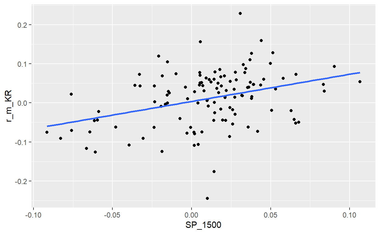
BT 20.17.2. Peter wants to add a low-beta stock to his portfolio. One candidate is Kroger’s stock (ticker: KR). As a proxy for the market, he uses the S&P 1500. He wrangled gross monthly returns for KR and SP_1500 over ten years such that his sample size is 120 pairwise returns. The regression results are displayed below.

Peters wants to make two decisions. In both cases, his test is a two-sided hypothesis test with 99.0% confidence. In the first test, the null hypothesis is that KR’s beta is zero. In the second test, the null hypothesis is that KR’s beta is one (1.0). Based on these regression results, which of the following is TRUE as a valid inference?

KR <- tq_get('KR',
               from = "2009-01-01",
               to = "2020-01-01")

SP1500 <- tq_get('SPTM',
               from = "2009-01-01",
               to = "2020-01-01")

KR <- KR %>% select(date, adjusted)
SP1500 <- SP1500 %>% select(date, adjusted)

KR_monthly <- KR %>% 
  tq_transmute(select = adjusted, mutate = to.monthly, indexAt = "lastof")
SP1500_monthly <- SP1500 %>% 
  tq_transmute(select = adjusted, mutate = to.monthly, indexAt = "lastof")

KR_monthly <- KR_monthly %>% mutate(
  r_m_KR = log(adjusted/lag(adjusted)))

SP1500_monthly <-SP1500_monthly %>% mutate(
  r_m_SP = log(adjusted/lag(adjusted)))

KR_monthly <- KR_monthly %>% 
  rename(date_KR = date,
         adj_KR = adjusted)

SP1500_monthly <- SP1500_monthly %>% 
  rename(date_SP = date,
         adj_SP = adjusted)

both_monthly <- cbind(SP1500_monthly, KR_monthly)

# testing different relationships really for Q&A properties
# both_131 <- both_monthly[-1, ]
both_120 <- both_monthly[-c(1:12), ]
# both_108 <- both_monthly[-c(1:24), ]
# both_96 <- both_monthly[-c(1:36), ]
# both_84 <- both_monthly[-c(1:48), ]
# both_72 <- both_monthly[-c(1:60), ]

both_120 <- both_120 %>% rename(SP_1500 = r_m_SP)
saveRDS(both_120, "t2-20-17-kroger-sp1500.rds")

con <- url("http://frm-bionicturtle.s3.amazonaws.com/david/t2-20-17-kroger-sp1500.rds")
both_120 <- readRDS(con)
close(con)

both_120 %>% ggplot(aes(x = SP_1500, y = r_m_KR)) +
  geom_point() +
  geom_smooth(method = "lm", se = FALSE)

model_120 <- lm(r_m_KR ~ SP_1500, data = both_120)
summary(model_120)


Call:
lm(formula = r_m_KR ~ SP_1500, data = both_120)

Residuals:
      Min        1Q    Median        3Q       Max 
-0.255113 -0.039050  0.009397  0.043573  0.203206 

Coefficients:
            Estimate Std. Error t value Pr(>|t|)    
(Intercept) 0.003594   0.006433   0.559    0.577    
SP_1500     0.696484   0.169073   4.119 7.08e-05 ***
---
Signif. codes:  0 '***' 0.001 '**' 0.01 '*' 0.05 '.' 0.1 ' ' 1

Residual standard error: 0.06775 on 118 degrees of freedom
Multiple R-squared:  0.1257,    Adjusted R-squared:  0.1183 
F-statistic: 16.97 on 1 and 118 DF,  p-value: 7.082e-05

###

model_120_tidy <- tidy(model_120)

gt_table_model_120 <- gt(model_120_tidy)

gt_table_model_120 <- 
  gt_table_model_120 %>% 
  tab_options(
    table.font.size = 14
  ) %>% 
  tab_style(
    style = cell_text(weight = "bold"),
    locations = cells_body()
  ) %>% 
  tab_header(
    title = "Kroger (KR) versus S&P_1500: Gross (incl. Rf) monthly log return",
    subtitle = md("Ten years (2010 - 2019), n = 120 months")
  ) %>% 
  tab_source_note(
    source_note = "Source: tidyquant https://cran.r-project.org/web/packages/tidyquant/"
  ) %>% cols_label(
    term = "Coefficient",
    estimate = "Estimate",
    std.error = "Std Error",
    statistic = "t-stat",
    p.value = "p value"
  ) %>% fmt_number(
    columns = vars(estimate, std.error, statistic),
    decimals = 4
  ) %>% fmt_scientific(
    columns = vars(p.value),
  ) %>% 
  tab_options(
    heading.title.font.size = 14,
    heading.subtitle.font.size = 12
  )

gt_table_model_120

Kroger (KR) versus S&P_1500: Gross (incl. Rf) monthly log return
Ten years (2010 - 2019), n = 120 months
Coefficient	Estimate	Std Error	t-stat	p value
(Intercept)	0.0036	0.0064	0.5587	5.77 × 10⁻¹
SP_1500	0.6965	0.1691	4.1194	7.08 × 10⁻⁵
Source: tidyquant https://cran.r-project.org/web/packages/tidyquant/

Third question

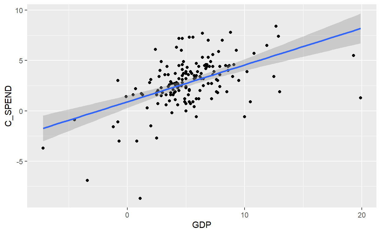
BT 20.17.3. Debra is an economist who is interested in the relationship between consumer spending and the gross domestic product (GDP). From the FRED database at the Fed’s Bank of St. Louis (https://fred.stlouisfed.org/) she collects quarterly data from 1980 through the first quarter of 2020; her series includes n = 161 quarters of data. She regresses consumer spending (C_SPEND), as the response (aka, dependent) variable against GDP as the explanatory (aka, independent) variable. Each series is not a level, but rather a seasonally adjusted percent change. The regression results are displayed below.

library(alfred)
library(ggplot2)


# startdate <- "1980-01-01"
# enddate <- "2020-01-01"
# startdate1 <- "1980-01-01"
# enddate1 <- "2020-01-01"

# gdp <- get_fred_series("A191RP1Q027SBEA", "GDP", observation_start = startdate1, observation_end = enddate1)
# cspend <- get_fred_series("DPCERL1Q225SBEA", "C_Spend", observation_start = startdate1, observation_end = enddate1)
# testing
# cdebt <- get_fred_series("CDSP", "C_Debt", observation_start = startdate1, observation_end = enddate1)
# df1 <- cbind(gdp, cdebt)
# df1 <- df1[-3]

# df2 <- cbind(gdp, cspend)
# df2 <- df2[-3]
# df2 <- df2 %>% rename(C_SPEND = C_Spend)
# saving dataframe because series data changed in the meantime!
# saveRDS(df2, "t2-20-17-spend-versus-gdp.rds")

con <- url("http://frm-bionicturtle.s3.amazonaws.com/david/t2-20-17-spend-versus-gdp.rds")
df2 <- readRDS(con)
close(con)

ggplot(df2, aes(GDP, C_SPEND)) + 
  geom_point() + 
  geom_smooth(method = "lm")

model_spend <- lm(C_SPEND ~ GDP, data = df2)
summary(model_spend)


Call:
lm(formula = C_SPEND ~ GDP, data = df2)

Residuals:
     Min       1Q   Median       3Q      Max 
-10.0025  -1.1513   0.2266   1.2048   4.6900 

Coefficients:
            Estimate Std. Error t value Pr(>|t|)    
(Intercept)  0.89995    0.31555   2.852  0.00492 ** 
GDP          0.36591    0.04993   7.329 1.11e-11 ***
---
Signif. codes:  0 '***' 0.001 '**' 0.01 '*' 0.05 '.' 0.1 ' ' 1

Residual standard error: 2.155 on 159 degrees of freedom
Multiple R-squared:  0.2525,    Adjusted R-squared:  0.2478 
F-statistic: 53.71 on 1 and 159 DF,  p-value: 1.107e-11

df_fit_tidy <- tidy(model_spend)

sd(df2$GDP)

[1] 3.411722

sd(df2$C_SPEND)

[1] 2.484429

cor(df2$GDP, df2$C_SPEND)

[1] 0.5024882

beta <- df_fit_tidy$estimate[2]
beta_r <- round(beta,4)
sd_gdp <- round(sd(df2$GDP),3)
sd_spend <- round(sd(df2$C_SPEND),3)
correlation_compute <- beta_r * sd_gdp/sd_spend

gt_table <- gt(df_fit_tidy)

gt_table <- 
  gt_table %>% 
  tab_options(
    table.font.size = 14
  ) %>% 
  tab_style(
    style = cell_text(weight = "bold"),
    locations = cells_body()
  ) %>% 
  tab_header(
    title = "Consumer Spending (C_SPEND) regressed against Gross Domestic Product (GDP)",
    subtitle = md("Quarterly Growth (Seasonally adjusted), 1980 to 2020:Q1, n = 161")
  ) %>% 
  tab_source_note(
    source_note = md("Source: FRED at https://fred.stlouisfed.org/")
  ) %>% cols_label(
    term = "Coefficient",
    estimate = "Estimate",
    std.error = "Std Error",
    statistic = "t-stat",
    p.value = "p value"
  ) %>% fmt_number(
    columns = vars(estimate, std.error, statistic),
    decimals = 4
  ) %>% fmt_scientific(
    columns = vars(p.value),
  ) %>% 
  tab_options(
    heading.title.font.size = 14,
    heading.subtitle.font.size = 12
  )

gt_table

Consumer Spending (C_SPEND) regressed against Gross Domestic Product (GDP)
Quarterly Growth (Seasonally adjusted), 1980 to 2020:Q1, n = 161
Coefficient	Estimate	Std Error	t-stat	p value
(Intercept)	0.9000	0.3156	2.8520	4.92 × 10⁻³
GDP	0.3659	0.0499	7.3285	1.11 × 10⁻¹¹
Source: FRED at https://fred.stlouisfed.org/

df_fit_tidy$p.value[2]

[1] 1.106954e-11

y_intercept <- df_fit_tidy$estimate[1]
se_y_intercept <- df_fit_tidy$std.error[1]
ci_confidence = 0.95
z_2s <- qnorm((1 + ci_confidence)/2)

ci_lower <- y_intercept - se_y_intercept*z_2s
ci_upper <- y_intercept + se_y_intercept*z_2s
ci_lower

[1] 0.2814779

ci_upper

[1] 1.518425

slope_c <-df_fit_tidy$estimate[2]
se_slope <- df_fit_tidy$std.error[2]
slope_ci_lower <- slope_c - se_slope * z_2s
slope_ci_upper <- slope_c + se_slope * z_2s
slope_ci_lower

[1] 0.2680529

slope_ci_upper

[1] 0.463775