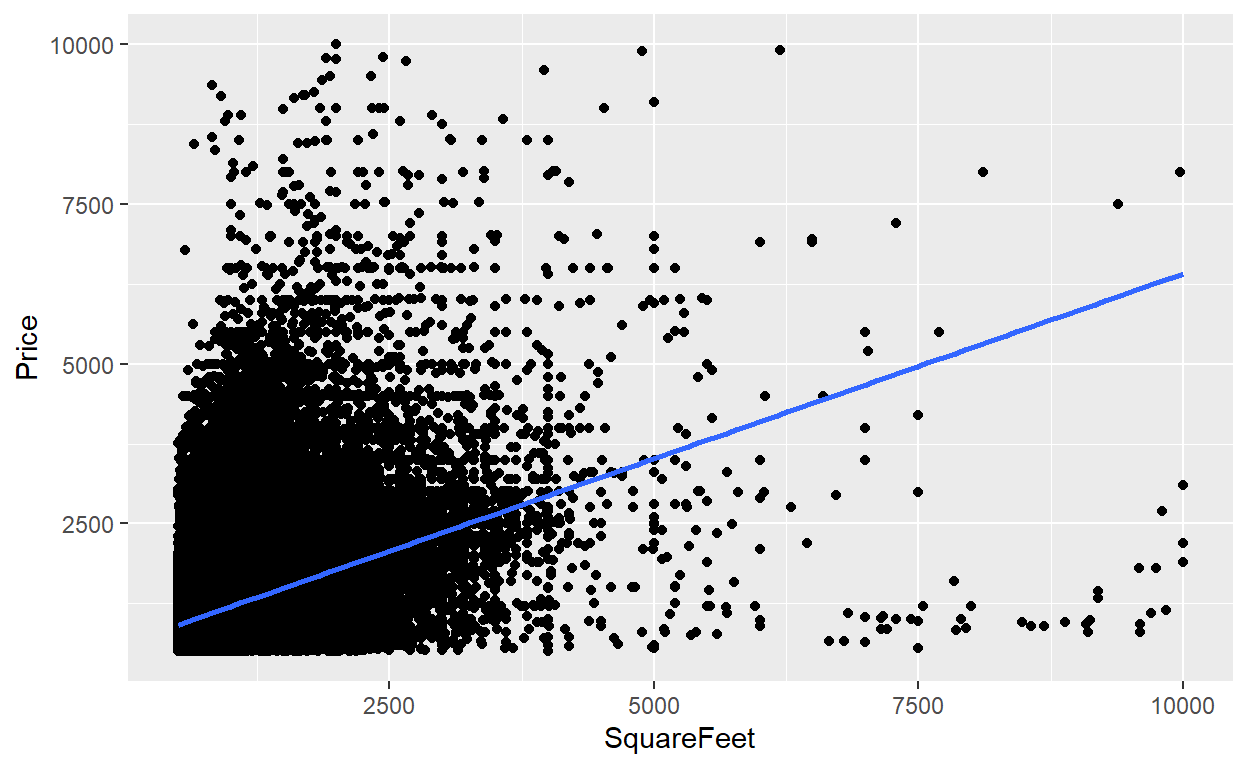
20.16.3. Sally works at a real estate firm and was asked by her client to quantify the relationship between rental size (in square feet) and rental price. She explained to her client that the relationship is multivariate but, given that caveat, she offered to perform a linear regression with a single explanatory variable. She retrieved a massive dataset (n = 360,400 observations and includes rentals across the United States) and regressed monthly rental price (aka, the explained variable) against rental size as measured by square feet. To illustrate the units, one of data points in the dataset is (y = $1,200 per month, X = 1,000 feet^2). The results are displayed below.
library(tidyverse)
library(gt)
library(broom)

# rentals_raw <- read_csv("housing.csv")
# rentals_sort <- rentals %>% arrange(price)
# rentals_df1 <- rentals_raw %>% filter(price > 500, price < 10000,
#                                       sqfeet> 500, sqfeet < 10000)
# boxplot(rentals$price)
# boxplot(rentals$price)$out
#
# rentals_df1 <- rentals_df1 %>% rename(
#  "Price" = "price",
#  "SquareFeet" = "sqfeet")
#
# saveRDS(rentals_df1, "rentals-sm.rds")

con <- url("http://frm-bionicturtle.s3.amazonaws.com/david/rentals-sm.rds")
rentals_df1 <- readRDS(con)
close(con)

model1 <- rentals_df1 %>% lm(Price ~ SquareFeet, data =  .)
summary(model1)
Call:
lm(formula = Price ~ SquareFeet, data = .)

Residuals:
    Min      1Q  Median      3Q     Max
-5382.8  -325.1  -122.7   185.9  8262.4

Coefficients:
             Estimate Std. Error t value Pr(>|t|)
(Intercept) 624.42303    2.59775   240.4   <2e-16 ***
SquareFeet    0.57889    0.00239   242.2   <2e-16 ***
---
Signif. codes:  0 '***' 0.001 '**' 0.01 '*' 0.05 '.' 0.1 ' ' 1

Residual standard error: 545.4 on 360399 degrees of freedom
Multiple R-squared:   0.14, Adjusted R-squared:   0.14
F-statistic: 5.866e+04 on 1 and 360399 DF,  p-value: < 2.2e-16
price_avg_act <- mean(rentals_df1$Price)
size_ave_act <- mean(rentals_df1$SquareFeet)
new.df.rentals <- data.frame(SquareFeet = c(1000, 1500, 1800, 2000, 2500))
predict(model1, new.df.rentals)
       1        2        3        4        5
1203.313 1492.758 1666.425 1782.203 2071.648
model1_tidy <- tidy(model1)
gt_table_rentals <- gt(model1_tidy)
gt_table_rentals <-
gt_table_rentals %>%
tab_options(
table.font.size = 14
) %>%
tab_style(
style = cell_text(weight = "bold"),
locations = cells_body()
) %>%
tab_header(
title = "Monthly Rental PRICE regressed against Square Feet",
subtitle = md("Entire United States, n = 360,400 observations")
) %>%
tab_source_note(
source_note = "Source: USA Housing Listings @ kaggle https://www.kaggle.com/datasets"
) %>% cols_label(
term = "Coefficient",
estimate = "Estimate",
std.error = "Std Error",
statistic = "t-stat",
p.value = "p value"
) %>% fmt_number(
columns = vars(estimate, std.error, statistic),
decimals = 3
) %>% fmt_scientific(
columns = vars(p.value),
) %>%
tab_options(
heading.title.font.size = 14,
heading.subtitle.font.size = 12
)
gt_table_rentals
| Monthly Rental PRICE regressed against Square Feet | ||||
|---|---|---|---|---|
| Entire United States, n = 360,400 observations | ||||
| Coefficient | Estimate | Std Error | t-stat | p value |
| (Intercept) | 624.423 | 2.598 | 240.370 | 0.00 |
| SquareFeet | 0.579 | 0.002 | 242.206 | 0.00 |
| Source: USA Housing Listings @ kaggle https://www.kaggle.com/datasets | ||||
rentals_df1 %>% ggplot(aes(SquareFeet, Price)) +
  geom_point() +
  geom_smooth(method = "lm")